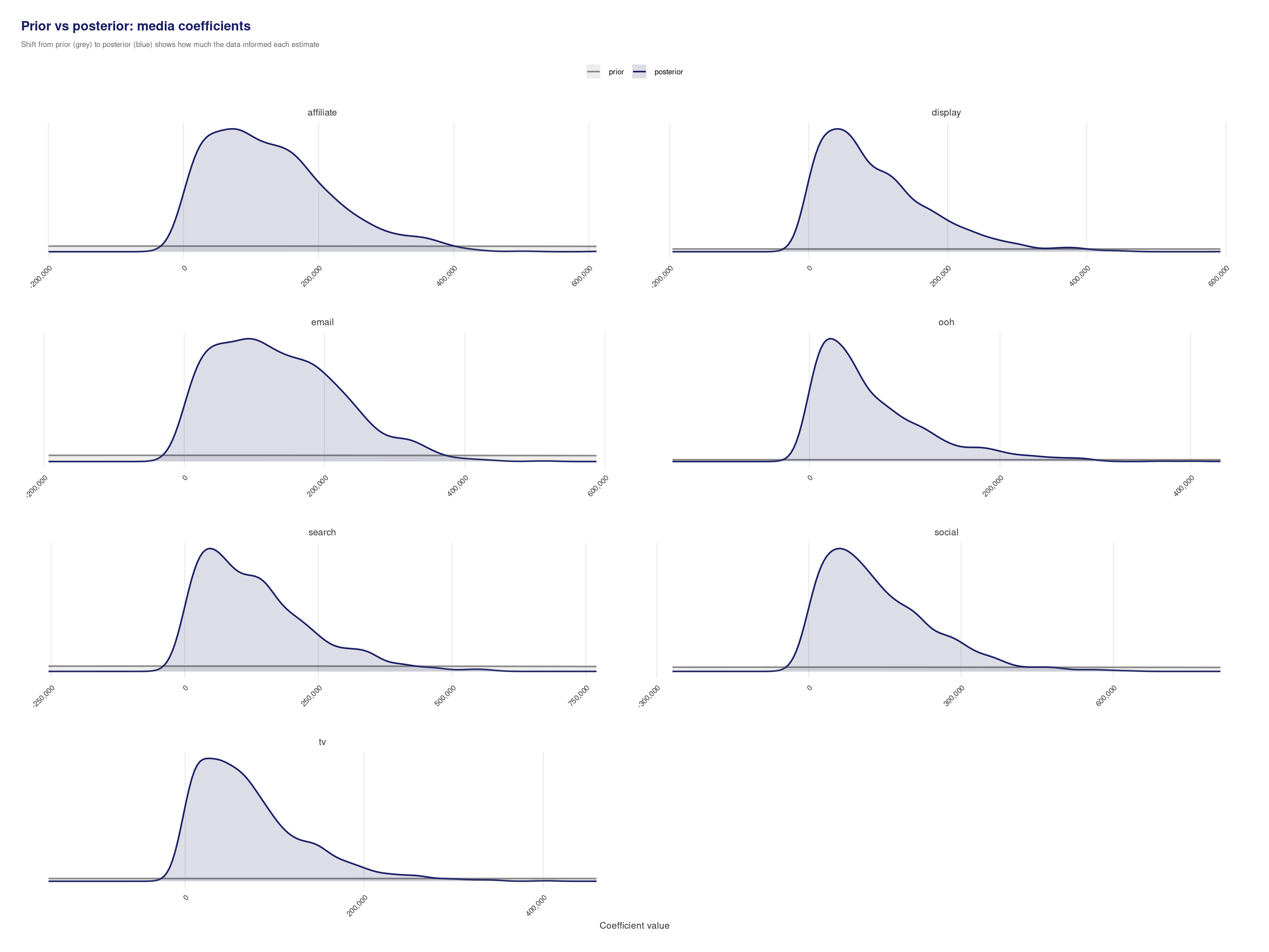
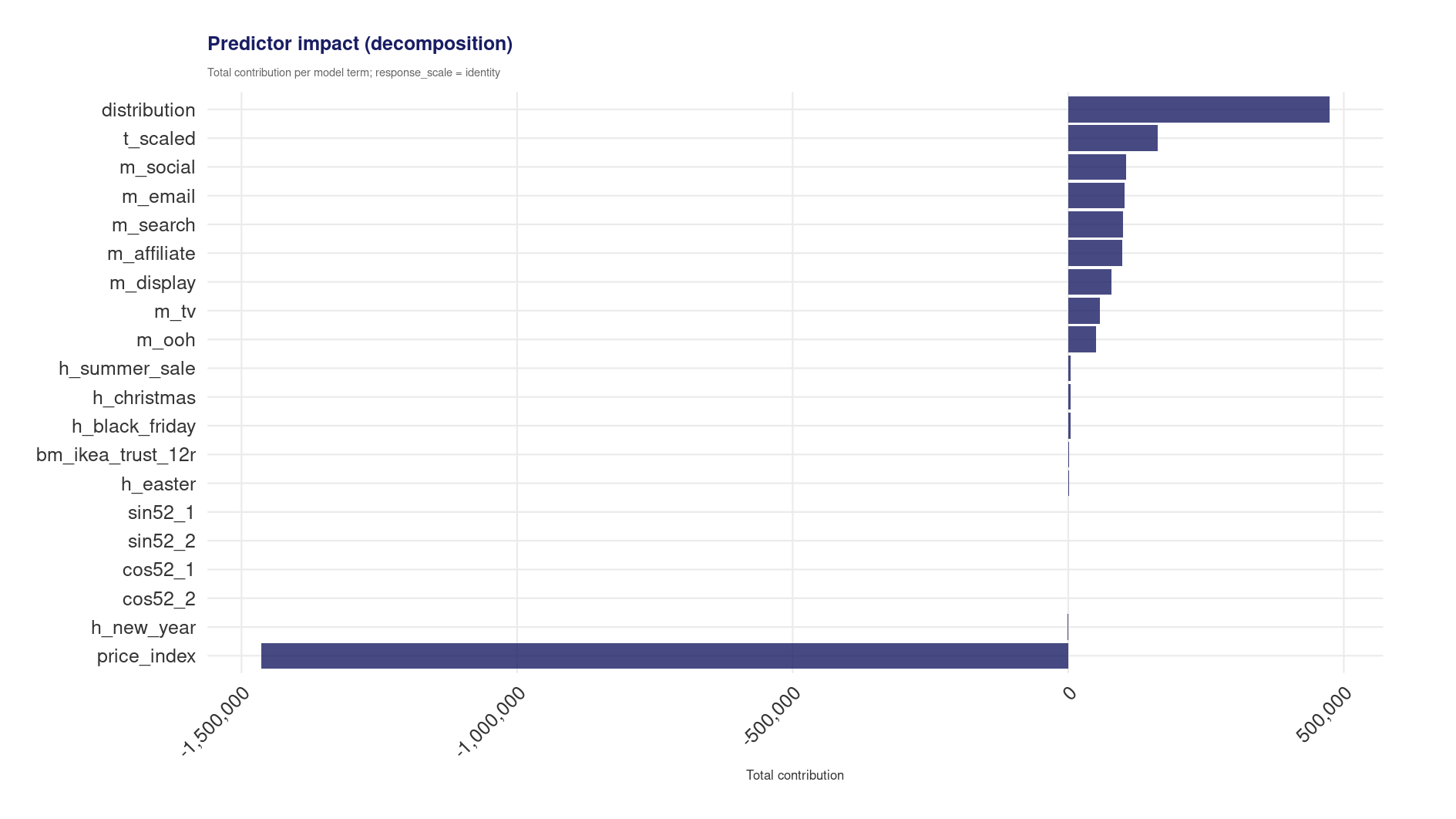
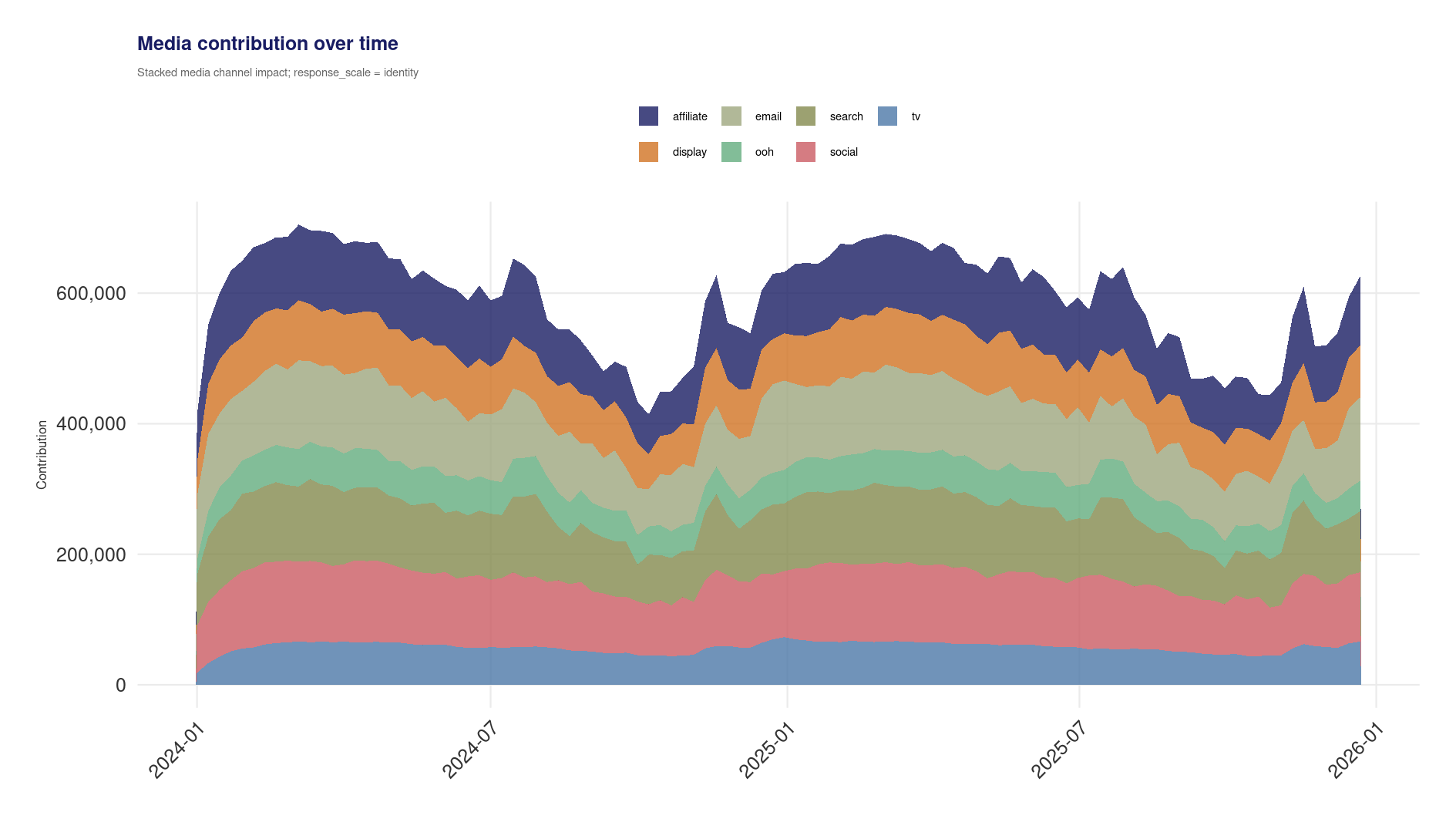
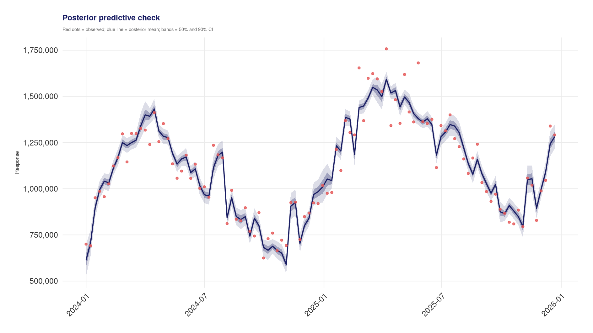
Documentation for DSAMbayes 1.3.5, a Bayesian marketing mix modelling toolkit for R, built on Stan.
DSAMbayes provides interfaces for single-market regression (BLM), multi-market hierarchical models with partial pooling, pooled models with structured media coefficients, and a bounded fixed-effects estimator. The fixed-effects API is coefficient-only and deliberately excludes the level-scale post-fit interfaces available to other model classes.
The docs are organised around a simple idea: DSAMbayes is not just an API or a runner. It is a way of operating a principled Bayesian MMM workflow with explicit assumptions, diagnostic gates, and decision rules.
If you are coming from OLS or frequentist MMM
Start with the workflow pages, not the YAML reference.
Are decomposition and optimisation outputs fit for use?
overall gate status plus uncertainty-aware reporting
Passing one row does not automatically imply the next row passes.
Support boundaries in 1.3.5
Supported workflows: BLM, RE, CRE, and pooled modelling; interactive R workflows; YAML runner validate and run; diagnostics; model selection; and budget optimisation.
Implemented but not qualified: the direct R fixed_effects() API supports Gaussian coefficient and residual-noise inference through MCMC plus within-contrast diagnostics. FE supports YAML runner validation, dry-run, and bounded MCMC fitting with a dedicated coefficient, sampler, within-design, contrast-residual, and contrast posterior-predictive artefact set. P4-J bounded technical gates passed for live runner execution, explicit-prior prior-only sampling, balanced and unbalanced one-replication recovery, and sampler diagnostics. This execution and regression evidence does not make the estimator production-qualified: it does not estimate repeated-sampling coverage or reliability. FE still rejects MAP, unit-intercept recovery, level prediction, generic model diagnostics, model selection, decomposition, counterfactual analysis, optimisation, forecasting, and deployment.
Supported with explicit limits: pooled models require MCMC, target.offset_column is supported only for model.type: blm, outputs.save_deployment_model_rds is supported for model.type: blm, for model.type: pooled with fit.method: mcmc, and for hierarchical model.type: re/cre with fit.method: mcmc, hierarchical deployment scoring is seen-groups-only, and time-series CV is not supported for pooled runs.
Reserved or limited surfaces: forecast currently creates only the 70_forecast/ stage with no forecast files or plots. Runner decomposition artefacts are linear term-contribution summaries and fail closed for hierarchical, offset-bearing, and probabilistic-media-transform models.
Changes in 1.3.5
Version 1.3.5 adds the bounded coefficient-only
fixed_effects() API and its bounded YAML validation, dry-run, fitting, and
artefact contract. Completed FE runs remain unqualified and do not enter the
generic level-scale or decision-layer pipeline. See Estimator
Capabilities for the exact execution
boundary and separately gated repeated-sampling qualification work.
The earlier v1.3.4 release introduced:
Posterior counterfactual response: aligned scenario and reference paths
can be evaluated with posterior uncertainty for supported fitted models.
Safer transformed-media handling: hierarchical row alignment and
single-channel Stan payload dimensions are preserved explicitly.
Clearer runner stages: scenario analysis uses
60_scenario_analysis/, forecasting remains reserved at 70_forecast/, and
optimisation uses 80_optimisation/.
Native decomposition: the external DSAMdecomp and teller path has
been removed; unsupported decomposition paths fail closed.
Estimator qualification remains gated by the estimator-methodology plan. An
implemented capability is not a production qualification.
Use Getting Started for setup, not for the whole methodology
The Getting Started pages are intentionally practical. Once you can run the package, use the workflow section to answer the two questions that matter most in Bayesian MMM:
how should I think about priors?
which diagnostics matter before I trust outputs?
Subsections of Getting Started
Install and Setup
Audience
Engineers and analysts setting up DSAMbayes for local development or modelling runs. This page is written for a Unix shell (Linux or macOS). If you are on Windows using RStudio, especially on a work-issued machine without full administrator rights, use Install and Setup (Windows / RStudio) instead.
Prerequisites
R >= 4.1: check with R --version.
A C++ toolchain for Stan compilation. This is the most common source of setup issues:
macOS: install Xcode Command Line Tools (xcode-select --install).
Windows: install Rtools matching your R version. Ensure make is on your PATH.
Linux (Ubuntu/Debian):sudo apt install build-essential.
# 1. Select an ABI-safe host library and create it with the cachesource scripts/r-library-path.sh
dsambayes_set_r_library host
mkdir -p "$R_LIBS_USER" .cache
# 2. Set the cache path (add both settings to .bashrc/.zshrc for persistence)exportXDG_CACHE_HOME="$PWD/.cache"# 3. Install DSAMbayes from the local checkoutR -q -e 'install.packages(".", repos = NULL, type = "source")'
This keeps all package libraries and Stan compilation caches inside the repo, avoiding permission issues with system library paths.
Do not share a compiled package library between R runtimes or containers.
dsambayes_set_r_library host selects
.Rlib-host-r<active-R-version>/; use dsambayes_set_r_library container
inside a container instead. The path is deliberately derived from the active
runtime, not hard-coded in the repository.
Verify the installation
1. Confirm DSAMbayes loads
R -q -e 'library(DSAMbayes); cat("Version:", as.character(utils::packageVersion("DSAMbayes")), "\n")'
If you need only the package API and have read access to the private canonical
repository, install it directly:
R -q -e 'remotes::install_github("tandpds/DSAMbayes-Charles-Dev", dependencies = NA, upgrade = "never")'
This installs the current package version from main. remotes reads
GITHUB_PAT from the environment for private-repository access. Keep the token
in your user environment or credential manager, never in a command, script, or
tracked file. Clone the repository instead when you need its example configs,
data, runme.R, or development tooling.
Using renv (optional)
The repository includes a renv.lock file for fully reproducible dependency management. To use it:
R -q -e 'install.packages("renv"); renv::restore()'
This installs the exact dependency versions used during development. It is optional but recommended for production runs where reproducibility matters.
Give new DSAMbayes users a compact conceptual orientation before they move into tutorials, runner usage, or the workflow section.
This page is intentionally introductory. It does not try to be the full methodology guide for Bayesian MMM. For that, use Principled Bayesian Workflow.
What is DSAMbayes?
DSAMbayes is an R package for Bayesian marketing mix modelling built on Stan. It provides:
an lm()-style modelling interface for interactive work
model classes for single-series, hierarchical, and pooled MMM
prior and boundary controls
post-fit extraction, diagnostics, decomposition, and optimisation tooling
a YAML/CLI runner for reproducible runs
The main practical difference from classical regression is that DSAMbayes works with a posterior distribution, not just a single fitted coefficient vector.
Why Bayesian MMM?
MMM datasets often have the exact features that make naive regression unstable:
short time series
overlapping media timing
strong baseline structure
uncertain functional form
real business need for uncertainty-aware decisions
Bayesian modelling helps because it makes several things explicit:
regularisation through priors
structural constraints through boundaries
uncertainty propagation into downstream outputs
diagnostic gates rather than fit-statistic-only thinking
The DSAMbayes mental model
DSAMbayes should be thought of as a workflow, not just a fitter.
At a high level:
specify the model and priors
fit the model
check whether the posterior computation is trustworthy
check whether the fitted model is adequate for the data
only then interpret decomposition, comparison, or optimisation outputs
That is the main philosophical shift from a simpler OLS-style workflow.
Model classes
DSAMbayes supports three main model classes.
BLM
Single-market Bayesian linear model.
Use when:
you have one KPI series
one market / brand / region is the modelling unit
you want the simplest Bayesian MMM starting point
Hierarchical
Multi-group model with partial pooling.
Use when:
you have panel data across markets, regions, or brands
you want to borrow strength across groups while preserving group structure
Pooled
Single-market model with structured pooling across labelled media dimensions.
Use when:
the outcome is one series
the media structure has nested or repeated dimensions that should share information
This walkthrough uses the tracked synthetic dataset at
data/timeseries/demo_data_synthetic.csv. It contains weekly observations for
a single series with columns for:
First-time Stan compilation takes 1–3 minutes. Subsequent runs use a cached binary. With the default 4 chains split across 2 cores, sampling on synthetic data typically completes in under 2 minutes.
Step 5: Sampler diagnostics
chain_diagnostics(fitted_model)
Metric
Good
Concern
Max Rhat
<= 1.01
> 1.01 means chains have not converged
Min ESS (bulk)
> 400
< 200 means too few effective samples
Divergences
0
Any non-zero count warrants investigation
These are the computational checks. They do not by themselves prove the model is adequate for interpretation.
Step 6: Extract the posterior
post<-get_posterior(fitted_model)
post is a tibble with one row per draw containing coef (named coefficient list), yhat (fitted values), noise_sd, r2, rmse, and smape.
$DecompedData shows each term’s contribution (coefficient × design-matrix
column) to the predicted KPI at each time point. The result is a native
dsambayes_decomposition S3 object.
Step 9: MAP for rapid iteration
During development, use MAP for fast point estimates:
Use MCMC for final reporting; MAP for formula iteration. A MAP result is one
point estimate, not posterior draws: it has no valid credible intervals or
MCMC diagnostics. Review the restart diagnostics if objectives differ
materially; use fit() when uncertainty, convergence, or decision risk
matters.
Common pitfalls
Pitfall
Symptom
Fix
Forgetting to set boundaries
Media coefficients go negative
Add set_boundary(m_x > 0)
Too few iterations
High Rhat, low ESS
Increase iter and warmup
Missing controls
High residual autocorrelation
Add trend, seasonality, or holiday terms
Scaling confusion
Coefficients look wrong
model.scale: true is default; get_posterior() back-transforms automatically
Build, fit, and interpret a multi-market hierarchical model with partial pooling and optional CRE (Mundlak) correction using the DSAMbayes R API.
This page is a hands-on tutorial. For the broader methodological questions behind prior-setting, diagnostics, and interpretation, use the workflow pages:
Boundaries apply to the population-level coefficients.
Step 3: (Optional) Add CRE / Mundlak correction
If you suspect that group-level spending patterns are correlated with
unobserved market characteristics (e.g. high-spend markets also have higher
baseline demand), CRE can model this correlation when the conditional mean of
the group effect is adequately represented by the included group means:
This adds one cre_mean_<channel> term for each media variable as a fixed
effect. Conditional on the CRE specification and other included controls, the
original media coefficient represents the within-group temporal association.
CRE does not solve omitted time-varying confounding or establish a causal
effect.
Hierarchical models are slower than BLM, expect 10–30 minutes depending on group count and data size. First-time Stan compilation of the hierarchical template adds 2–3 minutes.
Step 5: Check diagnostics
chain_diagnostics(fitted_model)
Pay special attention to Rhat and ESS for sd_* parameters (group-level standard deviations), which are often harder to estimate than population coefficients.
Step 6: Extract the posterior
post<-get_posterior(fitted_model)
For hierarchical models, coefficient draws from get_posterior() return vectors (one value per group) rather than scalars. The population-level (fixed-effect) estimates are averaged across groups.
Step 7: Group-level results
Fitted values and decomposition are returned per group:
# Fitted values, one row per observation, grouped by geofit_tbl<-fitted(fitted_model)head(fit_tbl)# Decomposition, per-group predictor contributionstbl_map<-data.frame(actual.vars=c("intercept","t_scaled","sin52_1","cos52_1","events","newsletters","cre_mean_channel0_signal","cre_mean_channel1_signal","cre_mean_channel2_signal","cre_mean_channel3_signal","channel0_signal","channel1_signal","channel2_signal","channel3_signal"),group=c(rep("BASE",10),rep("media",4)),ref_points=c("none",rep("mean",13)))decomp_result<-decomp(fitted_model,tbl_map=tbl_map)# One native decomposition result per retained group:head(decomp_result$decomp[[1]]$DecompedData)
Step 8: Budget optimisation (population level)
Budget optimisation uses population-level (fixed-effect) beta draws, not group-specific totals:
# See Budget Optimisation docs for full scenario specificationresult<-optimise_budget(fitted_model,scenario=my_scenario)
Key differences from BLM
Aspect
BLM
Hierarchical
Data structure
Single market
Panel (multiple groups)
Coefficient draws
Scalars
Vectors (one per group)
Fit time
2–5 min
10–30 min
Decomposition
Direct
Native result per retained geo; probabilistic media transforms are rejected
Forest/prior-posterior plots
Direct
Group-averaged population estimates
Stan template
bayes_lm_updater_revised.stan
general_hierarchical.stan (templated per group count)
Common pitfalls
Pitfall
Symptom
Fix
Too few groups
Weak partial pooling; group SDs poorly estimated
Need 4+ groups for meaningful hierarchical structure
Run from YAML, reproducible hierarchical runs via the runner
Quickstart (YAML Runner)
Goal
Complete one reproducible DSAMbayes runner execution from validation to artefact inspection, then load the fitted model in R to explore the results interactively.
This page is operational by design. It teaches you how to run the package, not the full modelling methodology. After the quickstart succeeds, use Principled Bayesian Workflow before treating outputs as decision-ready.
Complete the environment setup in Install and Setup (selecting the host library, creating the cache directory, and exporting XDG_CACHE_HOME) before continuing.
Usually 1 to 3 minutes. Subsequent runs typically reuse the cached binary. If compilation appears stuck, check the C++ toolchain in Install and Setup.
Do I need to set R_LIBS_USER every time?
Yes, unless you add it to your shell profile. Use
dsambayes_set_r_library host to select a repo-local path that is isolated
from both your system library and any container library.
Can I use renv instead of .Rlib?
Yes. The repo includes renv.lock. Use renv::restore() if you want exact dependency restoration.
Modelling
How many weeks of data do I need?
There is no hard minimum, but a useful rule of thumb is:
BLM: about 100+ weeks for a model with roughly 10 to 15 predictors
Hierarchical: about 80+ weeks per group, ideally with at least 4 groups
Shorter series can still be modelled, but the posterior will usually be much more prior-driven and less decision-ready.
Should I use identity or log response?
Identity when the KPI is naturally additive and variance is fairly stable
Log when the KPI is strictly positive and effect interpretation is more naturally multiplicative
If unsure, fit both and compare the adequacy and diagnostic picture, not just a single fit metric. See Response Scale Semantics.
add sparse sign constraints only for structural assumptions
add sparse prior overrides only when you can defend them in business or modelling terms
do not use priors as a substitute for weak model design
Where do prior numbers come from, and why aren’t they standardised like some other MMM tools?
Short answer: in DSAMbayes, you write priors in the original units of your
data, for example revenue, not in a standardised or z-score space. This is a
deliberate design choice, not a mistake, and it differs from some other MMM
tools, including Abacus, which ask you to specify priors directly in their
internal standardised space.
What “standardised space” means
Before Stan samples, most Bayesian MMM tools, DSAMbayes included, centre and
scale the response and predictors so the sampler works with unit-scale
quantities. This is a computational convenience: it improves sampler
efficiency and keeps step sizes well behaved across parameters with very
different natural magnitudes (e.g. revenue in the hundreds of thousands versus
a spend variable in the low thousands).
Where tools differ is which layer of that process they ask the user to think
in.
Abacus-style: you write the prior directly on the standardised space.
A config entry such as intercept: Normal(mu = 0, sigma = 2) is only
interpretable because Abacus has already decided how the target is scaled;
the 2 is “2 standard deviations of the standardised target”, not
“2 units of revenue”.
DSAMbayes: you write the prior on the original, reporting-scale units
of your data. intercept: Normal(mu = 120000, sigma = 15000) means
“baseline revenue is around 120,000, plus or minus roughly 15,000”, in
whatever currency or unit your target column uses. When model.scale: true
(the default), DSAMbayes converts this raw-scale prior into the correct
standardised parameterisation internally, fits, and then back-transforms
the posterior draws to your original units automatically. You never see or
touch the standardised numbers unless you set model.scale: false.
Both approaches produce equivalent underlying sampler behaviour. Neither is
“unscaled” in the sense of skipping standardisation; DSAMbayes just does not
require you to author priors in the post-scaling space.
Why DSAMbayes uses the reporting scale for the prior contract
The numbers stay checkable by a non-modeller. A stakeholder, or a
colleague reviewing your config, can look at
mu = 120000, sigma = 15000 and immediately judge whether that is a
sane assumption about baseline revenue. Nobody outside the modelling team
can sanity-check Normal(0, 2) on a standardised scale without first
recomputing what that implies in revenue terms.
The prior’s meaning does not silently drift between runs. A
standardised-space prior such as Normal(0, 2) means something different
each time you refit, because the underlying standard deviation used to
derive that scale changes with the data (different date range, different
market, a new data pull). A reporting-scale prior such as
Normal(120000, 15000) means the same thing, “baseline revenue is about
120k”, regardless of what the data’s standard deviation happens to be on
any given run. This avoids a common failure mode where a prior that looked
reasonable on one dataset becomes accidentally very informative, or
accidentally very diffuse, on the next.
It matches how priors are usually elicited in practice. Domain
knowledge about a KPI baseline, a channel’s plausible ROI, or a
competitor effect is almost always expressed in business units. Asking
the analyst to translate that into a standardised space by hand is an
extra, error-prone step that this design avoids.
This is consistent with standard Bayesian workflow guidance (see
What Principled Means and
Stage 2: Model and Priors): elicit
priors where you have real, defensible intuition, and let the software
handle re-parameterisation for computation.
What actually happens under the hood
DSAMbayes’s internal scaling of priors and boundaries, including the exact
transformation ratios for slopes, the intercept, and hierarchical group-level
standard deviations, is fully documented in
Priors and Boundaries under “Scale
semantics”. That page is the technical reference; this FAQ entry is only the
“why”.
How to sanity-check a prior you have written
Reason about it directly in your data’s natural units; that is what the
YAML priors: block and set_prior() both expect.
Use peek_prior(model) to see the full prior table on the reporting scale
before fitting.
If you want to see the internal standardised-space numbers DSAMbayes
actually passes to Stan, set model.scale: false on an otherwise identical
model and compare, or inspect the scaling terms directly; this is rarely
necessary for day-to-day modelling.
Do not manually convert your prior into a standardised space and enter that
instead. That would be double-scaling and will produce the wrong prior.
See also Minimal-Prior Policy for the
recommended default-first, sparse-override operating rule that this scaling
behaviour is designed to support.
How many MCMC iterations do I need?
The defaults are a reasonable starting point. Then inspect the Stage 4 diagnostics:
Rhat <= 1.01 and healthy ESS usually mean the draw count is adequate
Rhat > 1.01 or weak ESS usually means you need to increase iterations and warmup
any divergences should be addressed before treating the fit as decision-ready
How strict is the stationarity requirement for MMM?
DSAMbayes does not require the raw KPI to satisfy a textbook stationarity condition before fitting.
The important question is whether the remaining unexplained structure, after adding sensible controls and baseline terms, is weak enough that media effects are not standing in for missing baseline dynamics.
When should I set boundaries on media coefficients?
Use m_channel > 0 when non-negativity is a structural belief you would defend in writing. Do not apply blanket sign constraints just to make the output look tidier. See Stage 2: Model and Priors and Minimal-Prior Policy.
When should I use CRE (Mundlak)?
Use CRE when you want to separate within-group temporal effects from between-group cross-sectional structure in a hierarchical model. See CRE / Mundlak.
How should I handle CRE mean terms in decomposition / attribution?
Treat cre_mean_* terms as baseline or between-group structure, not as media attribution terms. They are there to absorb confounding structure, not to claim channel contribution.
What priors should I use on CRE mean terms?
Usually the defaults. Avoid manually tightening or positivity-constraining them unless you have a very strong reason, because that can undermine the whole point of CRE adjustment.
Can I add random slopes for CRE mean terms?
No. Those terms are constant within group, so random slopes on them are not separately identifiable from the group intercept.
What does scale = TRUE do?
It standardises the response and predictors before Stan fitting to improve sampler efficiency. Post-fit coefficient extraction is back-transformed automatically.
Runner and outputs
How long does a typical run take?
Roughly:
BLM MCMC: a few minutes
BLM MAP: seconds
Hierarchical MCMC: tens of minutes depending on size
Pooled MCMC: usually between BLM and hierarchical
First-time Stan compilation adds extra startup time.
What is the difference between validate and run?
validate checks config and data contracts without compiling or fitting Stan
run validates, fits, writes staged artefacts, and runs diagnostics
Always validate first after config changes.
Where do outputs go?
Under results/<timestamp>_<model_name>/ by default. See Output Artefacts.
How do I compare two model runs?
Use compare_runs() or compare the model-selection artefacts directly. See Compare Runs.
That is more important than memorising one threshold in isolation.
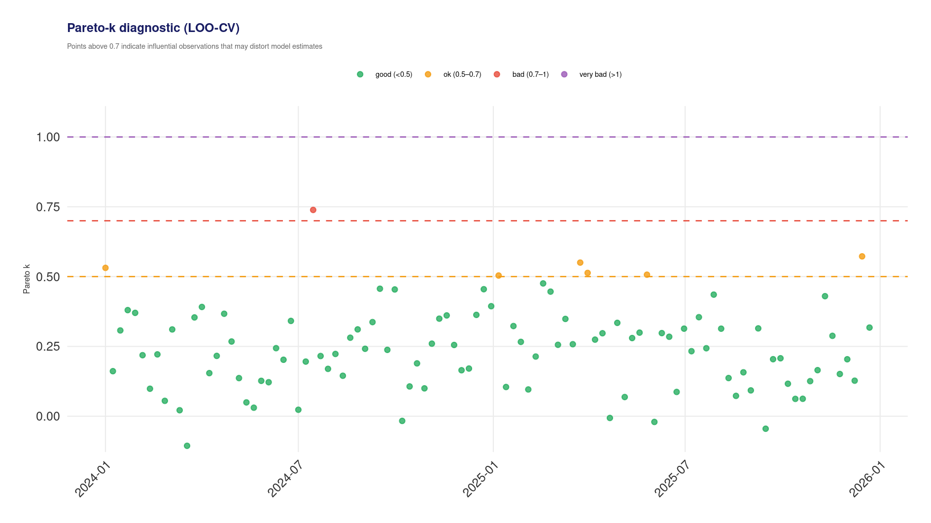
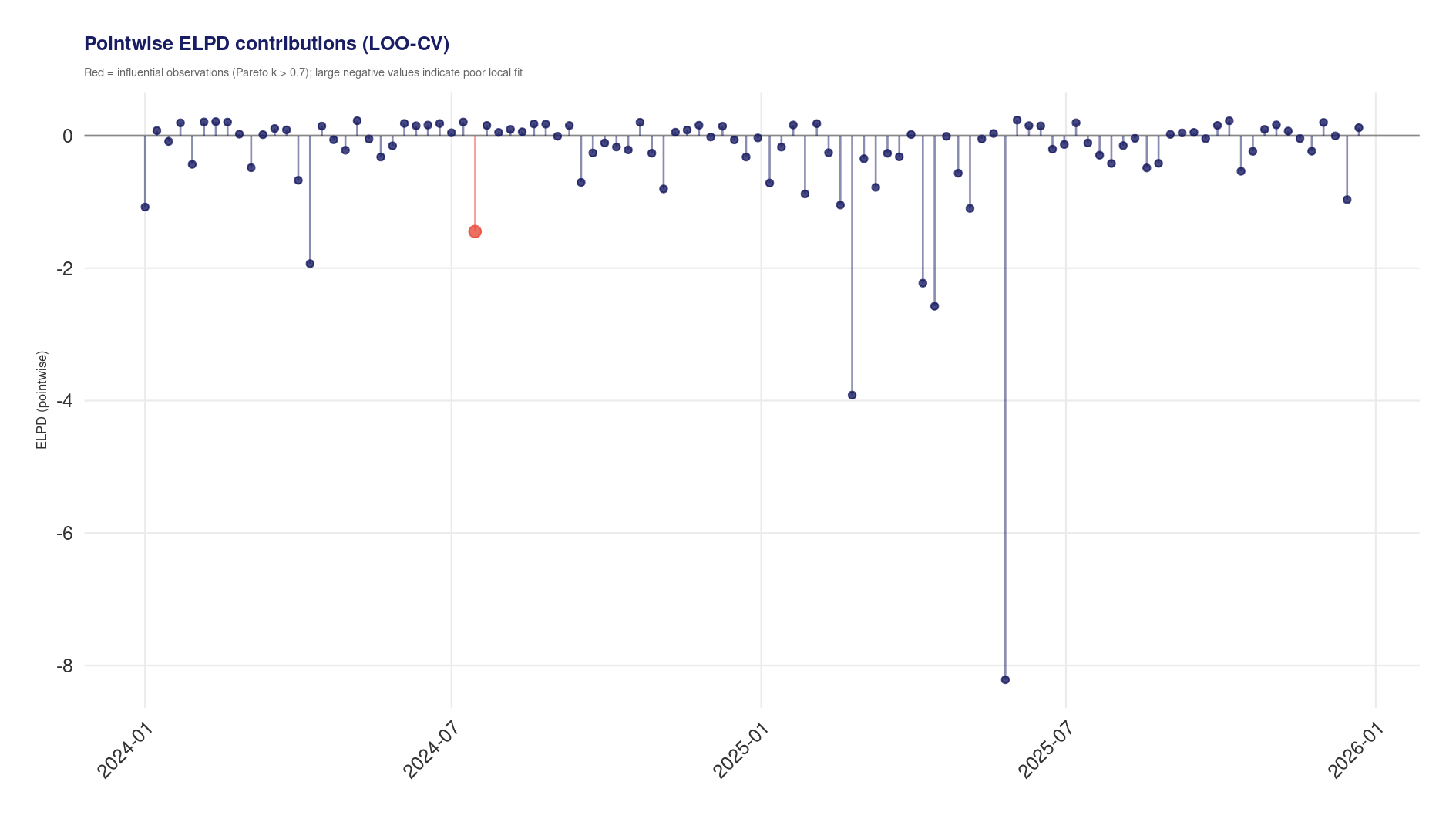
What does “Pareto-k > 0.7” mean?
It means the LOO approximation is unreliable for that observation and the point is highly influential. Investigate the observation and be cautious about using LOO-based comparisons mechanically.
My diagnostics say warn. Should I worry?
Usually yes, but not always in the same way.
in exploratory work, a warning may be acceptable if understood
in shareable reporting, warnings should be disclosed and interpreted
repeated or severe warnings usually mean the model needs revision before decision use
It searches feasible spend allocations within channel constraints and scores them against the fitted model. It is a decision layer built on the model, not an independent source of truth.
Can I use budget optimisation with MAP-fitted models?
Yes, but then the result is point-estimate-driven rather than uncertainty-rich. That is fine for rough iteration, not ideal for final decision support.
Principled Bayesian Workflow
Purpose
Give DSAMbayes users a workflow-shaped mental model for Bayesian MMM. This section is the methodological spine of the docs: it explains the sequence of decisions, assumptions, and diagnostic gates that should sit behind any DSAMbayes run.
Audience
Econometricians moving from OLS or other frequentist MMM workflows into Bayesian modelling.
Analysts who know how to run DSAMbayes but want a more defensible modelling process.
Reviewers who need to understand what a “good” DSAMbayes run should have passed before interpretation.
Why this section exists
DSAMbayes already documents its runner, model classes, priors, and diagnostics in detail. What most users still need is a clear answer to:
What is the modelling workflow?
Where do priors come from?
Which diagnostics matter most?
When is interpretation allowed, and when should it stop?
This section answers those questions directly. Use it before reading the lower-level reference pages.
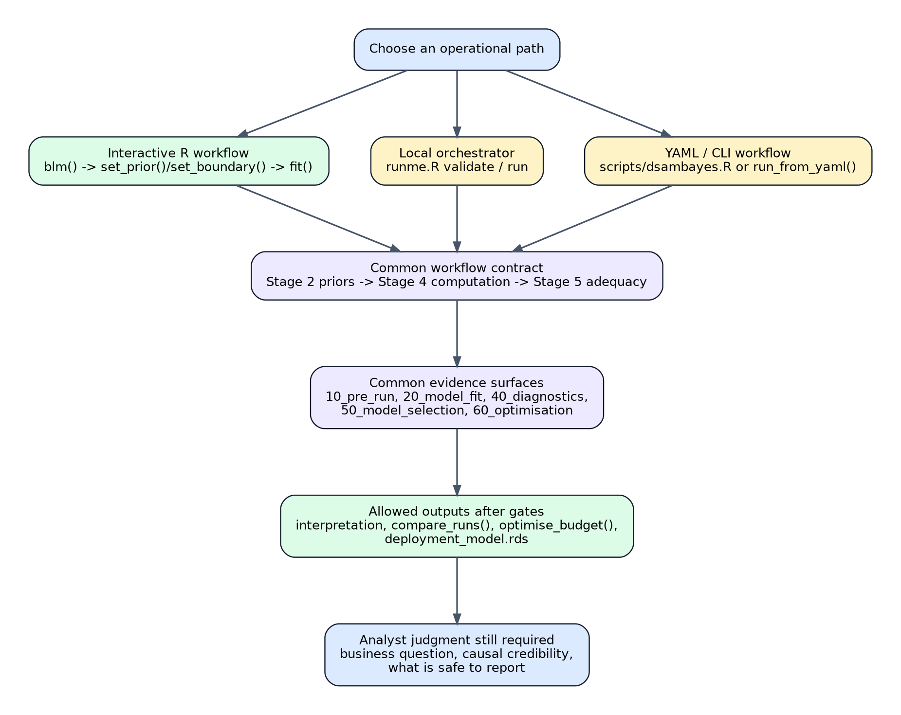
Workflow vectors
Different operational entry points in DSAMbayes still converge on the same
workflow contract. Whether you work interactively in R, use runme.R, or run
the YAML / CLI path, the result should still pass the same prior, computation,
and adequacy gates before interpretation.
fit plots, PPC, residual diagnostics, LOO/Pareto-k
Do not use decomposition or optimisation for decisions
Interpretation and decision
Are we reporting uncertainty and caveats honestly?
decomposition, response curves, optimisation
Restrict or block business use
Two rules to remember
1. Passing sampler diagnostics is necessary, not sufficient
Good Rhat, ESS, and zero divergences mean the posterior draws are numerically credible. They do not prove the model is a good description of the data, and they do not prove causal validity.
2. Good fit is not causal proof
A model can fit well, calibrate well, and still estimate the wrong media effects if the identifying assumptions are weak. DSAMbayes can make the workflow more disciplined; it cannot remove the need for analyst judgment.
How this section relates to the rest of the docs
Workflow pages answer “what should I do and why?”
How-to pages answer “how do I perform this task right now?”
Reference pages answer “what exactly does this field, function, or plot mean?”
Define what DSAMbayes means by a principled Bayesian MMM workflow.
The term is intentionally about process, not brand loyalty to a particular model class or sampler. A principled workflow is one where assumptions are explicit, diagnostics are stage-gated, and downstream interpretation is conditioned on those gates.
The short definition
A DSAMbayes workflow is principled when it does all of the following:
states a clear modelling objective and decision context
specifies an explicit model with explicit priors and boundaries
checks whether the posterior computation is trustworthy
checks whether the fitted model is adequate for the data
carries uncertainty and gate status into decomposition, optimisation, and reporting
If any one of those steps is skipped, the workflow becomes less defensible even if the final coefficients look plausible.
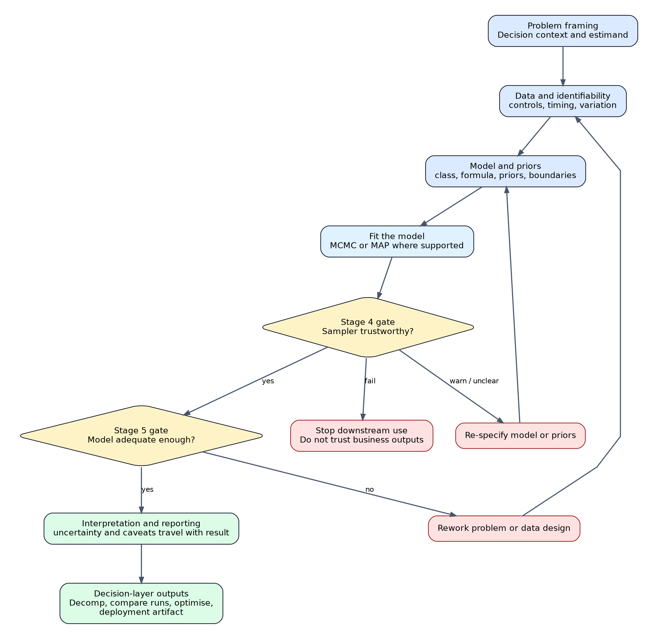
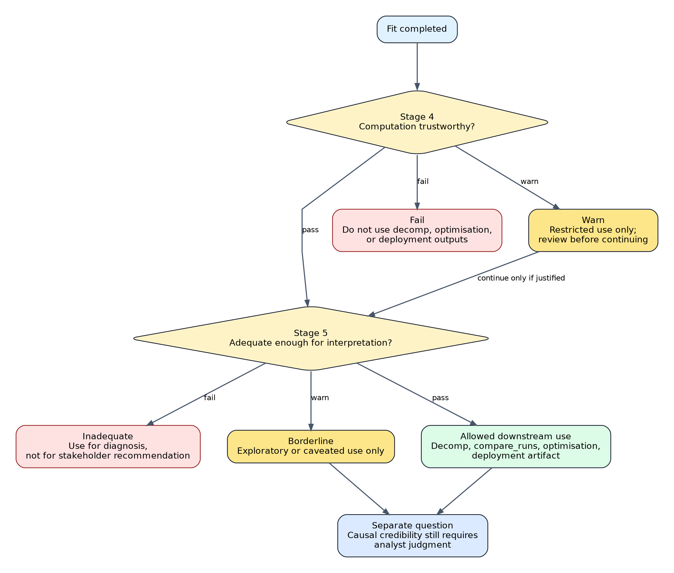
Workflow contract at a glance
The key design choice in DSAMbayes is that downstream outputs are conditional on
upstream gates. A model that fits is not automatically a model that should be
decomposed, compared, optimised, or deployed.
Four commitments
1. Generative transparency
The model should tell a clear story about how the outcome is generated from:
media terms
baseline structure
controls
observation noise
That is why DSAMbayes exposes priors, boundaries, response scale, CRE terms, time components, and model classes explicitly. The point is not to burden users with knobs; it is to make assumptions inspectable.
2. Stage-gated inference
The workflow should move in order:
question and data design
model and priors
fit
computational diagnostics
model adequacy checks
interpretation and decision support
Downstream outputs should only be trusted if the upstream gates have been checked.
3. Diagnostic sufficiency for computation, not causality
Diagnostics answer questions like:
did the sampler converge?
are the posterior draws stable?
does the fitted model describe the observed data credibly?
Diagnostics do not answer:
did the model identify the true causal effect of media?
did we control for every relevant confounder?
is the chosen baseline structure the only defensible one?
This distinction is essential in MMM.
4. Decision-linked reporting
Decomposition shares, response curves, deployment artifacts, and budget recommendations should be treated as functions of the gated fit, not as standalone truths. If the fit has warnings or failures, those limitations must travel with the result.
The three layers of trust
DSAMbayes users should separate three different questions:
Layer
Question
Typical evidence
Computational faithfulness
Are the draws numerically trustworthy?
Rhat, ESS, divergences, treedepth, BFMI
Model adequacy
Does the model describe the observed data credibly?
Passing the first layer does not imply the second. Passing the second does not imply the third.
How DSAMbayes supports this workflow
DSAMbayes already provides several pieces of the workflow contract:
explicit model classes and response-scale semantics
default priors plus selective overrides and hard boundaries
pre-flight design checks
post-fit diagnostics with pass / warn / fail statuses
staged runner artifacts under results/
model comparison and optional time-series selection tooling
decision-layer optimisation with uncertainty-aware summaries
What the package cannot do automatically is replace analyst judgment about:
business estimands
causal assumptions
whether a structural prior is genuinely defensible
whether a warned run is acceptable for the specific business use
Failure policy in plain language
If Stage 4 fails
Do not trust decomposition, response curves, or optimisation outputs. The posterior sample itself is numerically unreliable.
If Stage 5 fails
The sampler may have worked, but the model is not yet adequate for business interpretation. Use the run for diagnosis, not for stakeholder recommendations.
If causal assumptions are weak
Even a clean computational and adequacy profile may still only support associational interpretation. Report it that way.
Translate familiar classical regression instincts into the DSAMbayes workflow so users coming from OLS, GLM, or general frequentist econometrics can adopt Bayesian MMM without losing methodological discipline.
What does not change
Moving to DSAMbayes does not remove the need for:
careful data definition
sensible controls
thinking about omitted variables
residual scrutiny
skepticism about causal claims
Bayesian MMM is not a shortcut around model design. It is a different way of expressing assumptions and uncertainty.
What changes
1. From one best coefficient to a posterior distribution
In OLS, the default object of interest is a point estimate plus a standard error.
In DSAMbayes, the default object is a posterior distribution. That means:
coefficients are uncertain objects, not fixed truths
decomposition and optimisation should inherit that uncertainty
wide intervals are information, not a nuisance to hide
2. From “no prior” to “explicit prior assumptions”
Frequentist workflows often treat themselves as prior-free. In practice, they still encode structure through model choice, variable transformations, and constraints.
DSAMbayes makes that structure explicit:
default priors express mild regularisation
boundaries express structural sign assumptions
overrides should be sparse and justified
3. From significance-thinking to decision-thinking
The key question becomes less “is beta significantly different from zero?” and more:
is the posterior sufficiently stable?
is the model adequate?
is the interval narrow enough for the business decision?
what risks remain if we act on this estimate?
Quick translation table
Frequentist instinct
DSAMbayes replacement
“Run the regression and inspect coefficients”
Specify the model, priors, and boundaries, then inspect the full posterior
“Use p-values to screen variables”
Use posterior intervals, sign stability, and workflow diagnostics
“Choose the model with the best fit statistic”
Choose among models that first pass diagnostics and then compare predictive evidence
“If the model converged, the answer is credible”
Convergence is only the computation gate; adequacy and interpretation are separate gates
“No prior means unbiased starting point”
Defaults are still assumptions; make them explicit and inspect whether they are defensible
“A high R-squared validates the model”
Fit can be good while causal interpretation remains weak
The priors question in frequentist language
The question “where do priors come from?” is often really one of these:
What assumptions am I already making implicitly?
Which assumptions deserve to be encoded explicitly?
Where do I have stable directional knowledge versus weak intuition?
For DSAMbayes, the practical default is:
start with package defaults
add boundaries only for structural signs you would defend in writing
add sparse prior overrides only for high-conviction terms
do not use priors to force a preferred answer out of weak data
Default priors are a sensible starting point, not proof that prior design is solved forever.
Mistake 2: using priors as a repair tool for poor design
If media terms are badly collinear with baseline structure or controls are missing, stronger priors may stabilise numerics without fixing the underlying modelling problem.
Mistake 3: treating warning-level diagnostics as a cosmetic issue
A warned run may still be usable, but only if the warning is understood and disclosed. The right response is not “the model ran, so ship it.”
Mistake 4: confusing predictive success with causal proof
A model can rank well by ELPD and still be causally fragile.
Practical recommendation
If you are used to classical MMM, use DSAMbayes in this order:
Specify a model that is explicit enough to be audited and simple enough to be defended.
For most DSAMbayes users, this stage is where the biggest conceptual shift happens. In classical MMM, the common instinct is to choose variables, run the regression, and worry about coefficient stability afterwards. In DSAMbayes, priors and boundaries are part of the specification from the start.
The operating rule
Use a default-first workflow unless there is a strong reason not to.
That means:
start with the package defaults
add sparse sign constraints only where the business logic is structural
add sparse prior overrides only where the prior story is stable and defensible
fit the model
inspect whether the posterior is still dominated by weak design rather than by a sensible prior choice
This is the same operating stance documented in Minimal-Prior Policy, but framed here as part of the modelling workflow rather than as a standalone policy page.
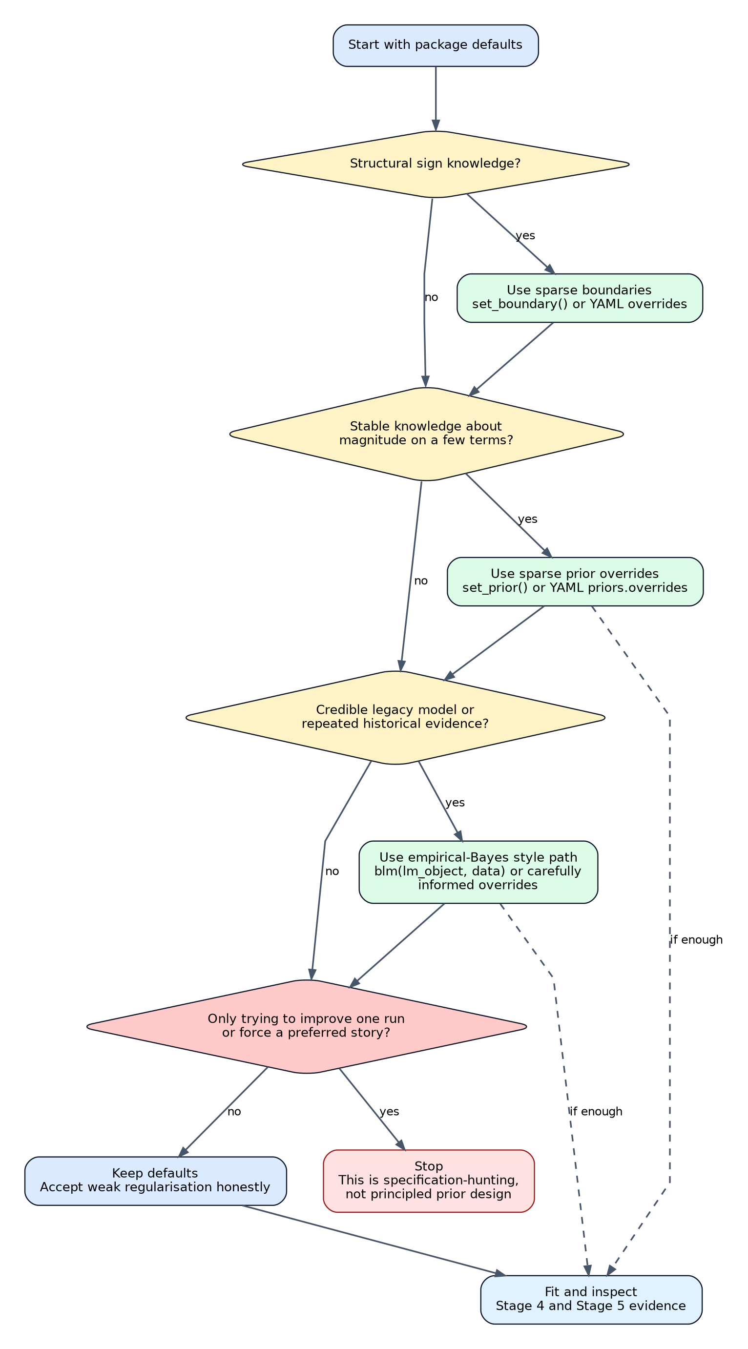
Prior specification pathways
This is the short answer to “where should priors come from?” Defaults are the
starting point. Boundaries and overrides are additive, sparse, and justified by
business or structural reasoning. The blm(lm_object, data) path is the
empirical-Bayes-like option when a credible legacy model already exists.
Where priors should come from
In DSAMbayes, priors should usually come from one of four sources.
1. Structural sign knowledge
Examples:
additional media exposure should not reduce KPI
competitor discount should not increase our sales
This is usually best expressed as a boundary, not as an aggressive mean-shifting prior.
2. Stable business knowledge about magnitude
Examples:
price elasticity is probably negative and modest
distribution is probably positive and not enormous
This is where a sparse override like normal(-0.2, 0.1) may be justified.
3. Historical learning from previous analyses
If the same brand, market, or response has been analysed repeatedly under a similar data-generating regime, you may have enough evidence to justify informative priors on a small number of terms.
4. Explicit regularisation when the data are weak
Sometimes priors are primarily there to stabilise a short, collinear MMM. That is acceptable, but it should be acknowledged honestly as regularisation rather than presented as deep subject-matter certainty.
Where priors should not come from
Do not set priors mainly because:
one previous run looked better with them
they remove a warning without improving model design
they force a preferred channel ranking
they make weak data look more certain than it really is
That is specification-hunting, not principled prior design.
Practical DSAMbayes policy
Step 1: start with defaults
For most first-pass BLM and hierarchical work, the package defaults are the right starting point.
default coefficient priors are weakly informative
default boundaries are unconstrained
you should not feel obliged to invent bespoke priors on every term
Step 2: add selective boundaries
Use set_boundary() or YAML boundaries.overrides when the sign is structural and defensible.
Good examples:
media terms constrained positive
competitor discount constrained non-positive
Poor examples:
constraining every control just to reduce posterior variance
forcing signs on variables whose mechanism is genuinely ambiguous
Step 3: add sparse prior overrides only where conviction is real
Typical candidates:
price
distribution
a small number of strategically important baseline controls
Typical non-candidates:
every media term
every generated seasonal component
every term simply because the data are noisy
Step 4: keep the reasoning on the original outcome scale
DSAMbayes can scale internally when scale = TRUE, but your reasoning about priors should still happen on the original business scale. Ask:
what outcome change would this prior imply?
would that be plausible for this KPI?
would I be comfortable defending it in a model review?
Prior predictive discipline in DSAMbayes
The Bayesian workflow ideal is to inspect prior implications before posterior fitting. In practical DSAMbayes use today, that discipline is still partly analyst-driven.
v1.3.3 does not yet provide a fully productised, first-class prior-predictive runner stage with its own public gate contract. So the current disciplined approach is:
keep the prior design simple
reason on the original outcome scale
avoid over-confident overrides unless they are well supported
fit the model and then inspect whether the posterior behaviour is compatible with the prior story and the data
That makes the lack of a first-class prior-predictive stage a reason to be more conservative, not less.
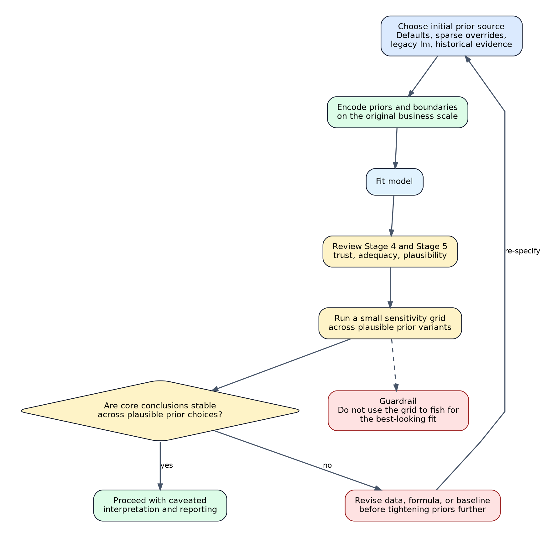
Prior calibration and sensitivity loop
For DSAMbayes users, a prior grid is a robustness tool, not a scoring contest.
Use it to check whether the substantive conclusion survives plausible prior
choices. Do not use it to hunt for the prior that makes one run look best.
How to know whether the priors are doing sensible work
After fitting, ask:
Are the intervals still wide?
If yes, the data may simply be weak. Do not respond automatically by tightening priors.
Are signs unstable without a clear design reason?
Check the baseline structure, controls, collinearity, and response-scale choice before strengthening priors.
Are coefficients pinned to hard bounds?
That can indicate that the boundary is too strong, or that the model is trying to express a structure the current formula does not support well.
A simple prior-setting decision table
Situation
Recommended action
First pass on a standard MMM
Use defaults, then add only obvious sign boundaries
Strong business reason for one control sign or magnitude
Add one sparse override or boundary
Weak identification and high collinearity
Diagnose design first; do not immediately tighten priors
Short dataset with many channels
Accept that intervals may stay wide; simplify model before forcing strong priors
Reviewer asks “why this prior?”
Be able to answer in one sentence on business or structural grounds
Decide whether the posterior draws are numerically trustworthy.
This stage is about computation quality, not business interpretation and not causal validity. If it fails, every downstream quantity that depends on posterior draws becomes unreliable.
The key question
Before asking whether the model is good, ask whether the sampler actually explored the posterior well enough for the summaries to mean what they appear to mean.
In DSAMbayes, this is the stage where you care most about:
divergences
Rhat
effective sample size
treedepth and BFMI when available
Recommended order of attention
1. Divergences
Any non-zero divergences should be treated seriously. They are often the strongest sign that the sampler struggled with posterior geometry.
Typical actions:
increase adapt_delta
simplify the model
revisit boundaries or extreme prior choices
inspect whether a hierarchical structure is too ambitious for the data
2. Rhat
Rhat answers: did the chains mix into the same posterior region?
Practical rule:
at or below 1.01 is the target
above 1.01 fails the publish and strict diagnostics policies
3. Effective sample size
ESS answers: how much independent information do the posterior summaries really contain after accounting for autocorrelation?
Low ESS means:
interval estimates may be unstable
tail probabilities may be noisy
apparent posterior precision may be misleading
4. Treedepth and BFMI
These are geometry warnings. They often indicate a difficult posterior shape even when Rhat looks acceptable.
What DSAMbayes gives you
You can inspect this stage through:
chain_diagnostics(model) for interactive fitted models
40_diagnostics/diagnostics_report.csv
40_diagnostics/diagnostics_summary.txt
diagnostics plots and residual artifacts produced by the runner
Decide whether the fitted model is a credible description of the observed data.
This is the stage that sits between computational trust and business interpretation. A model can pass sampler diagnostics and still fail here.
The key question
If I simulate from the fitted model, does it reproduce the important structure of the observed data well enough for decomposition, comparison, and optimisation to be taken seriously?
What to inspect first
1. Fitted-versus-observed behaviour over time
Ask:
does the model track the broad level and movement of the KPI?
are there long runs of systematic over- or under-prediction?
are key seasonal or event patterns still unexplained?
2. Posterior predictive checks
Posterior predictive plots tell you whether the fitted model can generate data that look like what you observed.
In DSAMbayes, this is the right way to think about the ppc.png artifact: not as decoration, but as an adequacy check.
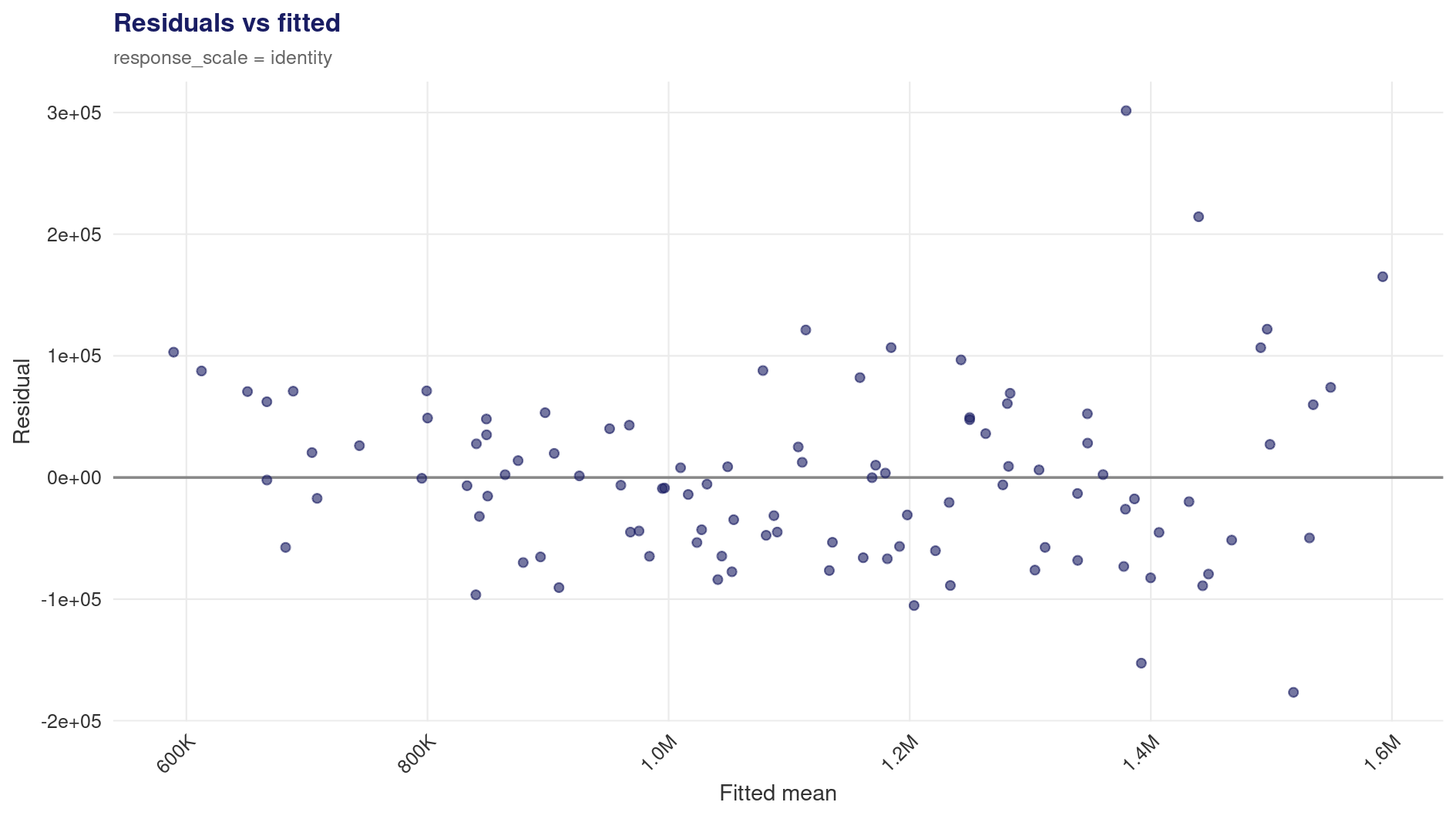
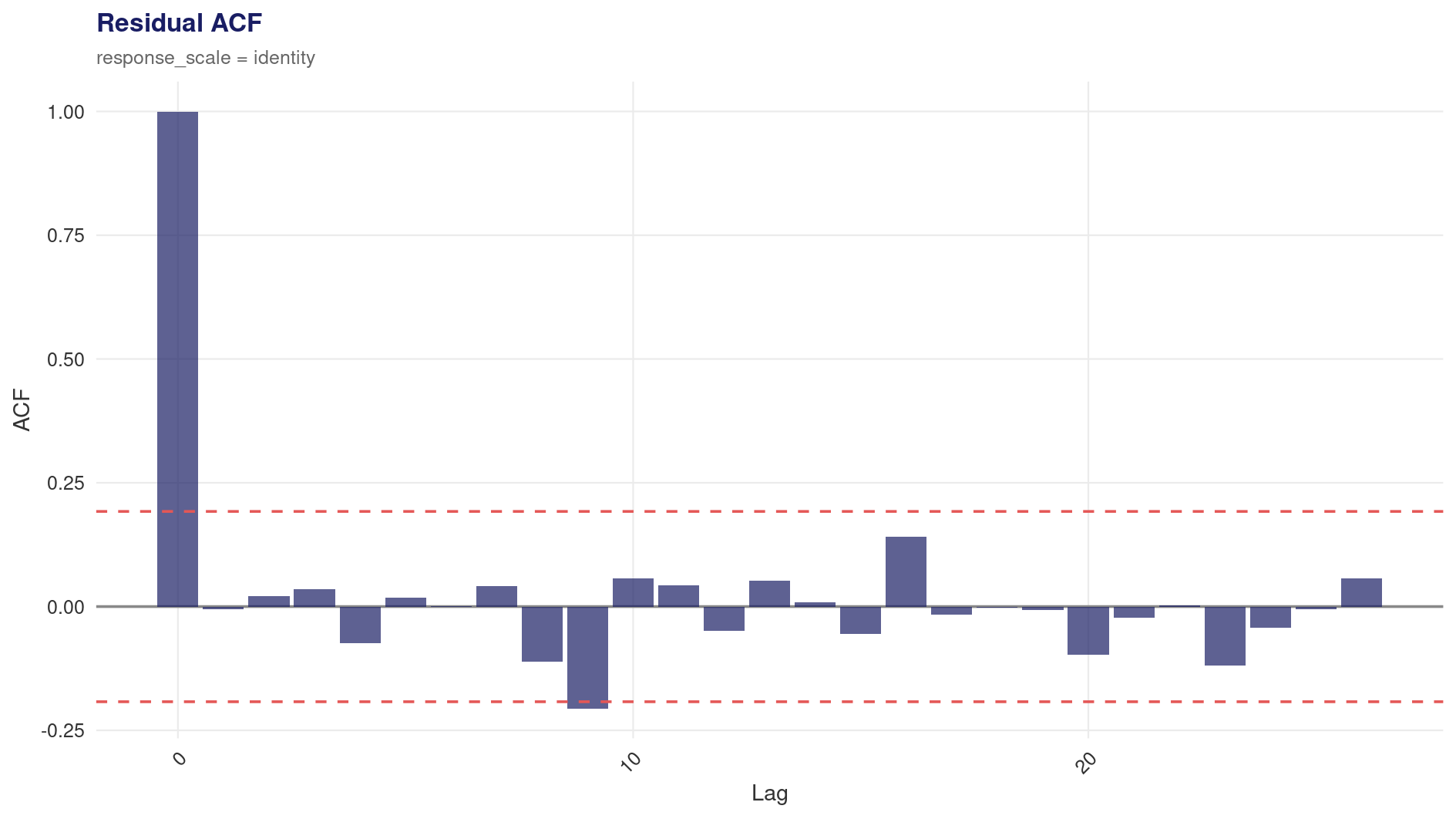
3. Residual behaviour
Residual autocorrelation or visible structure usually means the model has not absorbed an important baseline, timing, or event component.
4. LOO and Pareto-k
Model comparison and calibration-style plots help answer:
which candidate model predicts better?
are some observations highly influential?
is the leave-one-out approximation trustworthy?
These are useful, but they should not override a bad adequacy profile.
What this stage means for decisions
The main practical consequence of Stage 5 is that predictive ranking and
downstream business outputs are conditional on adequacy. Passing computation
checks is not enough if the fitted model still behaves poorly against the data.
If adequacy is poor
Do not interpret decomposition shares as if they were stable statements about media contribution.
Do not treat optimisation outputs as reliable budget guidance.
Use the run to diagnose misspecification, then revise the model.
If adequacy is acceptable but not clean
A warning-level result may still be useful for exploratory work, but the caveat should travel with the output.
Adequacy is not the same as causality
A model can:
fit well
calibrate well
compare well by predictive metrics
and still produce biased media-effect interpretation if confounding or structural misspecification remains.
So Stage 5 is a gate on model adequacy, not proof of causal validity.
Practical DSAMbayes reading order
Check Stage 4 first: are the draws trustworthy?
Inspect fit plots and PPC
Inspect residual diagnostics
Inspect LOO / Pareto-k and compare candidate runs
Only then interpret decomposition or decision-layer outputs
Common failure patterns
Pattern 1: good convergence, bad residual structure
Interpretation: the sampler worked, but the baseline or control structure is incomplete.
Pattern 2: good fit plot, unstable influential observations
Interpretation: apparent adequacy may depend too heavily on a small number of points. Treat model comparison and downstream interpretation cautiously.
Pattern 3: good predictive fit, weak causal story
Interpretation: the model may be operationally useful for forecasting or scenario analysis, but not for strong causal claims about media.
Ensure DSAMbayes is installed in the role-specific R_LIBS_USER selected by
dsambayes_set_r_library host.
Entry point
Rscript scripts/dsambayes.R <command> [flags]
Operational commands construct the package-owned
DSAMbayes::runner_cli_adapter() before reading configs, fitting models, or
writing artefacts. The startup panel records both the loaded package version
and the checkout version from DESCRIPTION. runme.R applies the same gate
and records the versions as package_version and checkout_version.
The versions must match exactly. A mismatch exits with status 2 before runner
work begins. Reinstall the current checkout into the active role-specific
library, then retry:
This gate proves declared-version equality. It cannot prove Git-revision
equality when the installed package has no revision metadata. Reinstall after
changing branches or pulling changes that keep the same package version. For a
CLI run, session_info.txt records the commit of the checkout that supplied
the entry-point script. This identifies the checkout; it does not independently
prove that a locally installed package with the same version contains identical
source bytes.
The script supports these commands:
init
validate
run
help (or -h / --help)
Command summary
Command
Required flags
Optional flags
Behaviour
init
--out
--template, --overwrite
Writes a config template file.
validate
--config
--run-dir
Runs config and data checks only (dry_run = TRUE).
run
--config
--run-dir
Executes the full pipeline (dry_run = FALSE) and writes run artefacts.
help
none
none
Prints usage text and exits.
Flag reference
init
--out <path> (required): output path for the generated YAML file.
--template <name> (optional): template name. Default is blm.
Supported values in script: master, blm, re, cre, pooled, hierarchical.
hierarchical maps to the same template file as re.
--overwrite (optional flag): allow overwrite of an existing --out file.
validate
--config <path> (required): YAML config path.
--run-dir <path> (optional): explicit run directory path.
run
--config <path> (required): YAML config path.
--run-dir <path> (optional): explicit run directory path.
Usage examples
Show help
Rscript scripts/dsambayes.R --help
Expected outcome: usage panel is printed with command syntax and notes.
Expected outcome: validation uses the provided run directory path when writing run metadata.
Execute full run
Rscript scripts/dsambayes.R run --config config/cre_geo_panel.yaml
Expected outcome: full modelling pipeline executes and artefacts are written under results/.
Execute full run with explicit run directory
Rscript scripts/dsambayes.R run \
    --config config/cre_geo_panel.yaml \
    --run-dir results/quickstart_run
Expected outcome: artefacts are written to results/quickstart_run (subject to overwrite rules in config).
Exit and error behaviour
Exit 0: command completed successfully. For run, this means the pipeline completed and diagnostics did not end in overall_status: fail.
Exit 1: run completed far enough to preserve the fitted result, but the outcome is non-publishable. This includes diagnostics overall_status: fail, requested scenario-analysis failures, diagnostics publish-gate failures, and post-fit artefact-write failures.
Exit 2: CLI argument, config, or runtime error before a completed run result could be returned.
Typical hard failures include:
DSAMbayes not installed.
Loaded DSAMbayes and checkout versions do not match.
Missing required flags (--out or --config).
Unknown command.
Unknown argument format.
Operational notes
validate is the recommended pre-run gate. Use it before run whenever you change config or data.
run prints a run summary and suggested next-step artefacts at completion.
The CLI itself does not define model semantics. Its package adapter delegates
execution to DSAMbayes::run_from_yaml().
Config Schema
Purpose
This page documents the authored YAML contract used by:
scripts/dsambayes.R
DSAMbayes::run_from_yaml()
runme.R
The authored schema is schema_version: 2 only. Older formula-driven YAML files are intentionally rejected.
Processing order
The runner processes configs in this order:
Parse YAML.
Coerce YAML infinity tokens (.Inf, -.Inf).
Apply v2 defaults.
Resolve relative paths against the config file directory.
Validate the authored v2 contract.
Compile the authored config into the internal runner config.
Apply managed holiday terms, then build the model and run.
Root sections
Key
Required
Purpose
schema_version
yes
Must be 2.
data
yes
Input data path, format, and date handling.
target
yes
Outcome column, KPI type, and response transform.
media
yes
Modeled media terms.
controls
yes
Non-media predictors, including manual trend/seasonality terms.
effects
no
Managed effects. In M1 this is holidays only.
model
yes
Model class and scaling options.
fixed_effects
conditional
Required exactly for model.type: fe.
hierarchy
conditional
Required for model.type: re and model.type: cre.
pooling
conditional
Required for model.type: pooled.
priors
no
Default priors plus grouped or explicit overrides.
boundaries
no
Grouped or explicit parameter boundaries.
fit
no
MCMC or optimise settings.
diagnostics
no
Diagnostics, model selection, and time-series selection settings.
allocation
no
Budget optimisation settings.
outputs
no
Output paths and artifact toggles.
forecast
no
Reserved forecast placeholder; currently only creates an empty stage directory when enabled.
Trend and seasonality stay user-authored as ordinary columns under controls.
Managed time effects are limited to holidays under effects.holidays.
re and cre models use hierarchy, not cre.enabled flags.
pooled models use pooling, not pooling.enabled.
fe models use fixed_effects.unit; hierarchy.group is not an FE alias.
Section reference
schema_version
Key
Type
Rules
schema_version
integer
Must be 2.
data
Key
Type
Rules
data.path
string
Required. File must exist. Relative paths resolve from the config directory.
data.format
string
csv, rds, or long.
data.date_var
string
Required in M1.
data.date_format
string or null
Optional parser format for date columns.
data.na_action
string
omit or error.
data.long_id_col
string or null
Required when data.format: long.
data.long_variable_col
string or null
Required when data.format: long.
data.long_value_col
string or null
Required when data.format: long.
data.dictionary_path
string or null
Optional metadata CSV.
data.dictionary
mapping
Optional inline metadata keyed by term name.
target
Key
Type
Rules
target.column
string
Required response column.
target.type
string
revenue or subscriptions.
target.transform
string
identity or log.
target.offset_column
string or null
Supported only for model.type: blm in M1.
media and controls
media is a required list of modeled media terms.
controls is a required list, but it may be empty ([]).
A term may not appear in both lists.
Manual trend and seasonality terms belong in controls.
All v2 names that become formula terms must be syntactic R names whose value is
preserved by make.names(). This rule applies to target.column,
target.offset_column, media, controls, fixed_effects.unit,
hierarchy.group, and generated term prefixes. ASCII names such as
sales_total and media.spend are the portable baseline. Non-ASCII names such
as média are supported only when the active R locale preserves the exact name
through make.names(). Rename columns containing spaces, operators, backticks,
or backslashes before using them in a v2 config; examples such as sales value,
paid-search, and sales`net are rejected during config validation. The
formula sentinels ., ..., and ..1-style pronouns are also rejected because
they do not evaluate as ordinary data columns.
Compiled formula order is:
generated holiday terms
controls
media
generated CRE mean terms
optional offset
hierarchical random-effects term
effects.holidays
Managed holidays are optional and are the only managed effect in M1.
Timezone used in parsing/alignment. Must be a valid Olson timezone such as UTC.
effects.holidays.prefix
string
Prefix for generated holiday columns.
effects.holidays.window_before
integer
Non-negative.
effects.holidays.window_after
integer
Non-negative.
effects.holidays.aggregation_rule
string
count or any.
effects.holidays.overlap_policy
string
count_all or dedupe_label_date.
effects.holidays.overwrite_existing
boolean
Replaces existing columns only when true.
Notes:
The data date column must be aligned to the configured weekly anchor.
Country filtering materializes a filtered calendar artifact before the compiled config is written.
model
Key
Type
Rules
model.name
string
Defaults to the config filename stem.
model.type
string
blm, fe, re, cre, or pooled.
model.scale
boolean
Controls internal scaling before fit.
model.force_recompile
boolean
Forces Stan recompilation when true.
fixed_effects
fixed_effects is required exactly when model.type: fe. The approved shape
has one unit key:
model:type:fescale:truefixed_effects:unit:geo
fixed_effects.unit must name one syntactic source column. It must differ from
the target, date, media, and control columns. For long-format data it must equal
data.long_id_col. FE configs cannot also contain hierarchy or pooling.
FE runner support includes validation, dry-run, and bounded non-dry MCMC
fitting. Validation and dry-run construct and pre-flight the same unfitted
fixed_effects model used by the direct API without Stan compilation or
sampling. A materialised dry-run writes only 00_run_metadata/. A non-dry run
uses the configured MCMC settings, the existing fit.fixed_effects() path, and
the dedicated FE artefact writer.
The FE-safe resolved defaults are:
Field
FE default or required value
data.na_action
error
target.transform
identity
fit.method
mcmc
fit.mcmc.parameterization.positive_priors
centered
diagnostics.model_selection.enabled
false
diagnostics.time_series_selection.enabled
false
diagnostics.identifiability.enabled
false
diagnostics.enforce_publish_gate
false
scenario_analysis.enabled
false
allocation.enabled
false
forecast.enabled
false
outputs.layout
staged
FE grouped priors support media_beta, control_beta, holiday_beta, and
noise_sd. Explicit prior overrides may target an authored slope or
noise_sd. Grouped boundaries support media_beta, control_beta, and
holiday_beta; explicit boundary overrides may target authored slopes only.
Intercept, CRE, pooling, random-effect, and residual-noise boundary requests
are rejected.
FE v1 also rejects offsets, log targets, MAP, non-centred positive priors,
internal media transformations, implicit row omission, scenario analysis,
allocation, forecasting, model selection, time-series selection, generic
identifiability output, publish-gate enforcement, flat output layout, level
fitted or residual output, deployment, decomposition, and optimisation.
The resolved config exposes save_within_design_csv,
save_contrast_residuals_csv, and save_contrast_ppc_csv for the dedicated FE
artefact stage. Contrast-space fitted values are diagnostics, not level-scale
fitted values or predictions. A completed FE run reports
qualification_status: not_assessed and does not set a publishability result.
No generic level-scale fitted, observed, residual, diagnostics, decomposition,
scenario, optimisation, model-selection, time-series-selection, forecast, or
deployment artefacts are written.
hierarchy
Required for model.type: re and model.type: cre.
Key
Type
Rules
hierarchy.group
string
Grouping column for panel models.
hierarchy.random_intercept
boolean
Include `(1
hierarchy.random_slopes
list of strings
Optional subset of authored media and controls.
hierarchy.cre_variables
list of strings
Required and non-empty for model.type: cre.
hierarchy.cre_prefix
string
Prefix for generated CRE mean terms. Default cre_mean_.
pooling
Required for model.type: pooled.
Key
Type
Rules
pooling.grouping_vars
list of strings
Required and non-empty.
pooling.map_path
string
Required. CSV or RDS.
pooling.map_format
string
csv or rds.
pooling.min_waves
integer or null
Optional positive integer.
priors
Key
Type
Rules
priors.use_defaults
boolean
Must remain true in M1.
priors.likelihood
mapping
Optional explicit alias for noise_sd.
priors.overrides
list
Explicit parameter-level overrides.
Grouped families are available when applicable:
intercept
media_beta
control_beta
holiday_beta
cre_beta
pooling_beta
random_effect_sd
noise_sd
Each grouped family accepts either the legacy DSAMbayes style:
family:normal # or lognormal_ms where supportedmean:0sd:0.5
or the more explicit alias:
distribution:Normal # or HalfNormal / LogNormalMS where supportedmu:0sigma:0.5
HalfNormal compiles to a zero-centered Normal prior plus an implied lower bound of 0 for unconstrained targeted parameter(s). Parameters that are already positive by construction, such as noise_sd and hierarchical sd_*[...], do not receive an extra boundary row.
Boundary families mirror the grouped prior families and may also use explicit boundaries.overrides.
Each grouped or explicit boundary row uses:
lower:-Infupper:Inf
For FE, grouped boundaries support media_beta, control_beta, and
holiday_beta. A boundary on noise_sd is not supported.
fit
Key
Type
Rules
fit.method
string
mcmc or optimise. Pooled runs require mcmc.
fit.seed
numeric or null
Optional scalar seed.
fit.optimise.*
mapping
Optimisation controls.
fit.mcmc.*
mapping
Stan sampling controls.
fit.mcmc.parameterization.positive_priors
string
centered or noncentered.
diagnostics
Retains the current runner surface for:
model_selection
time_series_selection
identifiability
publish-gate controls
Important M1 rule:
diagnostics.time_series_selection.enabled: true is not supported for pooled runs.
time-series selection is advisory only in the current release contract; it is not part of publish-gate enforcement.
lower-level runner paths with adstock/Hill media_transforms are not supported by time-series selection.
diagnostics.time_series_selection.gap_weeks is optional, defaults to 0, and inserts an embargo between the training window and the scored holdout window.
FE requires model selection, time-series selection, generic identifiability,
and publish-gate enforcement to remain disabled.
scenario_analysis
Opt-in posterior scenario/reference evaluation after a successful MCMC fit:
scenario_path and reference_path must identify CSV or RDS data frames.
Relative paths resolve from the config file directory.
Both inputs must contain aligned rows and all predictors, offsets, date fields,
and grouping fields required by the fitted model. They need not contain the
response column.
fit.method must be mcmc. MAP output does not provide posterior contrasts.
scale is response or kpi. For log-response models, log_response chooses
the lognormal conditional mean or the conditional median on the KPI scale.
aggregate_by names retained label columns. An empty list aggregates the full
supplied path within each draw.
save_draws: false writes summaries and metadata only. Set it to true to
add scenario_aggregate_draws.csv.
For fitted adstock/Hill media, the first supplied observation resets carry-over.
If decision-horizon values depend on known earlier exposure, prepend the same
observed history to both inputs. The runner reports every supplied row, so
retain a field that distinguishes warm-up rows from decision rows if needed.
The output is a model-implied fitted-response contrast, not automatic causal
attribution. See Counterfactual response.
allocation
Retains the current runner surface for budget optimisation, with channel targeting based on authored media terms.
allocation.n_candidates defaults to 2000 and must be a finite integer
from 10 through .Machine$integer.max.
allocation.posterior.draws defaults to 500 and must be a finite integer
from 1 through .Machine$integer.max.
Work scales approximately with candidates multiplied by retained posterior
draws and, for efficient frontiers, by the number of feasible budget levels.
See Budget Optimisation for measured review
thresholds and the benchmark command.
outputs
outputs.root_dir and outputs.run_dir behave as before, but the metadata contract now includes:
config.original.yaml
config.resolved.yaml
config.compiled.yaml
outputs.save_model_rds controls the full fitted analysis artifact 20_model_fit/model.rds
outputs.save_deployment_model_rds controls the compact deployment artifact 20_model_fit/deployment_model.rds
When outputs.overwrite: true targets an existing run directory, the runner
first validates the complete directory tree. It deletes only recognised flat
or staged artifact paths. Unknown files, nested directories, and symbolic links
cause an error before any existing artifact is deleted. Empty recognised stage
directories may remain and are reused. Concurrent mutation of a run directory
during overwrite is not supported.
Current first-slice limit:
outputs.save_deployment_model_rds: true is supported for model.type: blm, model.type: pooled with fit.method: mcmc, or hierarchical model.type: re / cre with fit.method: mcmc.
Pooled deployment artifacts score on authored terms and keep the normalized pooling map, but deployment-time newdata / data = ... does not need the pooling columns unless they are also ordinary formula terms.
Hierarchical deployment artifacts are seen-groups-only; explicit scoring/decomposition data must include the raw grouping columns, and decomposition also requires the response source column(s).
FE dry-runs write metadata only. Non-dry FE runs use bounded MCMC fitting and
may write the dedicated posterior summary, sampler text, within-design,
contrast-residual, and contrast posterior-predictive artefacts. They do not
enter generic post-fit or decision-layer paths and remain unqualified.
forecast
Reserved placeholder only. In v1.3.3, enabling forecast can materialise 70_forecast/, but the runner does not emit forecast files or plots.
Examples in this repository
config/blm_timeseries.yaml, weekly time-series BLM example
config/fe_panel.yaml, weekly geo-panel FE validation, dry-run, and bounded
MCMC example
config/re_geo_panel.yaml, weekly geo-panel RE example
config/cre_geo_panel.yaml, weekly geo-panel CRE example
outputs.layout: staged (default) writes files under numbered stage folders.
outputs.layout: flat writes all files directly under the run directory.
Stage folders used by the runner:
00_run_metadata
10_pre_run
20_model_fit
30_post_run
40_diagnostics
50_model_selection
60_scenario_analysis (only when scenario_analysis.enabled: true)
70_forecast (reserved; directory only when forecast.enabled: true)
80_optimisation (only when optimisation or allocation output is written)
artifact_schema_version: 2 identifies this layout. Schema-v1 run directories
retain 60_optimisation/; the runner does not rename historical results.
Command behaviour
validate
validate uses dry_run = TRUE.
If no run directory is resolved, no artefacts are written.
If a run directory is resolved (--run-dir or outputs.run_dir), config.original.yaml is written.
If a run directory is resolved (--run-dir or outputs.run_dir), config.resolved.yaml is written.
If a run directory is resolved (--run-dir or outputs.run_dir), config.compiled.yaml is written.
If a managed holiday country filter is active and a run directory is resolved, holiday_calendar.filtered.csv is materialised under 10_pre_run/.
If a run directory is resolved and outputs.save_session_info_txt: true, session_info.txt is written.
If forecast is enabled and a run directory is materialised, the 70_forecast/ directory is created.
run
run writes the full artefact set subject to config toggles and runtime conditions.
Fixed-effects run boundary
Fixed-effects (model.type: fe) runs use a dedicated artefact contract. They
fit the existing coefficient-only MCMC estimator, then return before the
generic post-fit and decision-layer paths.
With the tracked config/fe_panel.yaml defaults, a completed staged run writes:
00_run_metadata/artifact_schema.yaml
00_run_metadata/config.original.yaml
00_run_metadata/config.resolved.yaml
00_run_metadata/config.compiled.yaml
00_run_metadata/run_status.yaml
00_run_metadata/session_info.txt
20_model_fit/model.rds
30_post_run/posterior_summary.csv
40_diagnostics/chain_diagnostics.txt
40_diagnostics/diagnostics_summary.txt
40_diagnostics/within_design.csv
40_diagnostics/contrast_residuals.csv
40_diagnostics/contrast_ppc.csv
The relevant outputs.* flags may remove optional files from this inventory.
Setting outputs.save_posterior_rds: true adds
20_model_fit/posterior.rds. Managed holidays may add the existing holiday
provenance files under 10_pre_run/.
The two RDS files have different purposes. model.rds is the full fitted
same-environment analysis object; it preserves the fitted RStan state and
retained FE metadata for reload under the compatible R, RStan, and package
environment. posterior.rds is the optional compact extracted posterior table;
it is not an executable fitted model and does not replace model.rds.
posterior_summary.csv contains slopes and noise_sd; it does not contain a
unit intercept, RMSE, or SMAPE. The three contrast tables use the deterministic
orthonormal Helmert basis retained by the fitted model. Their values and labels
are basis-dependent diagnostics, not row-level observations, level-scale fitted
values, or predictions. Preserve contrast_label and contrast_basis when
comparing or joining these files.
diagnostics_summary.txt records factual design metadata and includes:
Therefore, a completed FE run makes no diagnostic pass, publishability, or
production-qualification claim. No generic level-scale fitted, observed,
residual, diagnostics, decomposition, scenario, optimisation, model-selection,
time-series-selection, forecast, or deployment artefacts are written.
Artefact contract by stage
00_run_metadata
File
Controlled by
Written when
Notes
config.original.yaml
always
run dir materialised
Raw YAML text from the input config.
config.resolved.yaml
always
run dir materialised
Authored config after defaults, path resolution, and v2 schema validation.
config.compiled.yaml
always
run dir materialised
Internal compiled runner config after the friendly YAML is translated into the downstream runtime shape.
artifact_schema.yaml
always
run dir materialised
Machine-readable runner artifact contract marker. Includes artifact_schema_version and the active artifact layout (staged or flat) so downstream tooling can reason about cross-version comparisons.
run_status.yaml
best-effort
run dir materialised
Machine-readable terminal run outcome. The runner attempts to write it for dry runs, fit failures after metadata creation, successful completions, scenario-analysis failures, diagnostics publish-gate failures, and post-fit artefact-write failures. Severe file-system failures can still prevent the file from being created.
session_info.txt
outputs.save_session_info_txt
flag is true
Includes DSAMbayes version, artifact schema version, config schema version, model/fit metadata, and sessionInfo().
10_pre_run
File
Controlled by
Written when
Notes
transform_assumptions.txt
outputs.save_transform_assumptions_txt
flag is true
Written even if transform sensitivity scenarios are disabled.
transform_sensitivity_summary.csv
outputs.save_transform_sensitivity_summary_csv
sensitivity object exists with rows
Requires transforms.sensitivity.enabled: true and successful scenario execution.
transform_sensitivity_parameters.csv
outputs.save_transform_sensitivity_parameters_csv
sensitivity object exists with rows
Parameter means/SD by scenario.
dropped_groups.csv
none
groups dropped by pooling.min_waves filter
Written only when sparse groups are excluded.
holiday_calendar.filtered.csv
none
managed holidays enabled with a country filter
Materialised filtered holiday calendar consumed by config.compiled.yaml.
holiday_feature_manifest.csv
none
managed holidays enabled and features generated
Documents generated holiday terms and active-week counts.
design_matrix_manifest.csv
outputs.save_design_matrix_manifest_csv
flag is true and manifest non-empty
Per-term design metadata.
data_dictionary.csv
outputs.save_data_dictionary_csv
flag is true and dictionary table non-empty
Merges inline YAML metadata and optional CSV dictionary metadata.
spec_summary.csv
outputs.save_spec_summary_csv
flag is true and table available
Single-row model/spec summary.
vif_report.csv
outputs.save_vif_report_csv
flag is true and predictors available
VIF diagnostics for non-intercept predictors.
20_model_fit
File
Controlled by
Written when
Notes
model.rds
outputs.save_model_rds
flag is true
Fitted model object.
deployment_model.rds
outputs.save_deployment_model_rds
flag is true and the fitted model is either model.type: blm, model.type: pooled with fit.method: mcmc, or hierarchical model.type: re/cre with fit.method: mcmc
Compact deployment artifact for explicit predict(newdata = ...) and explicit-data decomposition. It is additive to model.rds and does not replace the full analysis object. Pooled deployment artifacts retain authored-term scoring behaviour without shipping runtime dimension_map state. Hierarchical deployment artifacts are seen-groups-only; explicit prediction and decomposition data must include raw grouping columns, and decomposition also requires the response source column(s).
posterior.rds
outputs.save_posterior_rds
flag is true and MCMC fit
Raw posterior object for MCMC runs only.
fit_metrics_by_group.csv
implicit
fitted summary is computed
Written when any of save_fitted_csv, save_fit_png, save_residuals_csv, save_diagnostics_png is true.
fit_timeseries.png
outputs.save_fit_png
flag is true and ggplot2 installed
Observed vs fitted over time on the model response scale, with a subtitle that states the model form (levels or semilog), the displayed scale, fit metrics including Classical R^2 (posterior mean), and monthly date labels when date is a true Date.
fit_scatter.png
outputs.save_fit_png
flag is true and ggplot2 installed
Observed vs fitted scatter on the model response scale, with a subtitle that states the model form (levels or semilog) and the displayed scale.
posterior_forest.png
none
posterior draws available and ggplot2 installed
Posterior coefficient forest plot; skipped for optimise/MAP runs.
prior_posterior.png
none
posterior draws available, model has priors, and ggplot2 installed
Prior-versus-posterior comparison plot; skipped for optimise/MAP runs.
30_post_run
File
Controlled by
Written when
Notes
observed.csv
outputs.save_observed_csv
flag is true
Observed response on model response scale.
observed_kpi.csv
outputs.save_observed_csv
flag is true and response scale is log
KPI-scale observed values (exp) with conversion_method = point_exp.
fitted.csv
outputs.save_fitted_csv
flag is true
Fitted summaries on model response scale.
fitted_kpi.csv
outputs.save_fitted_csv
flag is true and response scale is log
KPI-scale fitted summaries (exp).
posterior_summary.csv
outputs.save_posterior_summary_csv
flag is true and MCMC fit
Posterior summaries for coefficients and scalar diagnostics.
decomp_predictor_impact.csv
outputs.save_decomp_csv
flag is true and runner linear term-contribution tables are supported
Predictor-level design column × posterior mean coefficient table. This is not the mapping/reference-point result returned by decomp(). Unsupported models produce a skip in artifact_status.csv.
decomp_timeseries.csv
outputs.save_decomp_csv
flag is true and runner linear term-contribution tables are supported
Long-format linear contribution-by-date table. Unsupported models produce a skip in artifact_status.csv.
decomp_predictor_impact.png
outputs.save_decomp_png
runner contribution tables are supported and ggplot2 is installed
Predictor-impact linear contribution plot.
decomp_timeseries.png
outputs.save_decomp_png
runner contribution tables are supported and ggplot2 is installed
Media linear-contribution time-series plot.
Active v1.3 pipeline note:
30_post_run/ emits observed and fitted summaries, posterior summaries, and runner linear term-contribution artefacts when their toggles are enabled.
Runner contribution artefacts fail closed for hierarchical models, models with offsets, and models fitted with probabilistic media transforms. Use the native interactive decomp() contract where that model class is supported.
When decomposition is unavailable, the runner records deterministic skip rows in 40_diagnostics/artifact_status.csv rather than silently dropping the contract entries.
40_diagnostics
File
Controlled by
Written when
Notes
chain_diagnostics.txt
outputs.save_chain_diagnostics_txt
flag is true and MCMC fit
Chain diagnostics text output.
diagnostics_report.csv
outputs.save_diagnostics_report_csv
flag is true and diagnostics object exists
One row per diagnostic check.
diagnostics_summary.txt
outputs.save_diagnostics_summary_txt
flag is true and diagnostics object exists
Counts by status and overall status.
estimator_checks.csv
none
the fitted model retains typed estimator checks
Stable estimator check IDs, severity, status, metric, threshold, and recovery action. Structural failure aborts before fitting, so a completed run records checks that reached pass or advisory warning.
row_reconciliation.csv
none
exact-frame reconciliation metadata exists
Input, retained, and excluded counts plus excluded source-row IDs and reason codes. It never contains response values.
cre_estimability_summary.csv
none
the fitted CRE model retains its preparation-time estimability report
Combined between-design rank and residual degrees of freedom plus separately labelled unweighted and group-size-weighted condition/VIF summaries. Each row records the ordered design terms, preparation policy, runner diagnostics mode, and diagnostic thresholds used.
cre_estimability_groups.csv
none
the fitted CRE model retains its preparation-time estimability report
Selected CRE grouping keys, prefixed with group_var_, and retained observation counts. It contains no response values.
cre_estimability_vif.csv
none
the fitted CRE model retains its preparation-time estimability report
Per-term VIF values for unweighted and group-size-weighted between designs. When fewer than two eligible predictors exist, each eligible predictor has an explicit not-applicable row.
cre_estimability_variation.csv
none
the fitted CRE model retains its preparation-time estimability report
Within-, between-, and total-variation evidence for each CRE variable, including exact-zero and near-zero flags and the active warning threshold.
cre_estimability_singular_values.csv
none
the fitted CRE model retains its preparation-time estimability report
Singular values, ranks, and tolerances for the combined between design and both centred predictor information designs.
hierarchy_support_summary.csv
none
a fitted RE or CRE model retains its preparation-time hierarchy support report
One row per random-effects block with group-size distribution, covariance dimension and groups-per-parameter evidence, advisory flags, and the active policy. Covariance support is reported without a threshold.
hierarchy_support_groups.csv
none
a fitted RE or CRE model retains its preparation-time hierarchy support report
Retained grouping keys, prefixed with group_var_, and observation counts for every random-effects block. It contains no response values because the response is structurally rejected from random-effect terms and grouping keys.
hierarchy_support_rank.csv
none
a fitted RE or CRE model retains its preparation-time hierarchy support report
Per-group random-effects design rank, residual degrees of freedom, singular-value bounds, and the active rank tolerance.
hierarchy_support_variation.csv
none
a fitted RE or CRE model retains its preparation-time hierarchy support report
Within-, between-, and total-variation evidence for every random slope, including exact-zero and near-zero flags.
artifact_status.csv
none
artifact status rows recorded by the runner
Per-artifact status log for skipped/warn/error events.
residuals.csv
outputs.save_residuals_csv
flag is true and fitted summary is computed
Residual table on response scale.
residuals_timeseries.png
outputs.save_diagnostics_png
flag is true and ggplot2 installed
Residuals over time.
residuals_vs_fitted.png
outputs.save_diagnostics_png
flag is true and ggplot2 installed
Residuals vs fitted.
residuals_hist.png
outputs.save_diagnostics_png
flag is true and ggplot2 installed
Residual histogram.
residuals_acf.png
outputs.save_diagnostics_png
flag is true and ggplot2 installed
Residual autocorrelation plot.
residual_diagnostics.csv
none
diagnostics residual checks available
Ljung-Box / ACF check outputs.
residuals_latent.csv
none
diagnostics latent residuals available
Latent residual series from diagnostics object.
residuals_latent_acf.png
outputs.save_diagnostics_png
latent residuals available and ggplot2 installed
Latent residual ACF plot.
ppc.png
none
posterior predictive plot available and ggplot2 installed
Posterior predictive check plot; skipped for optimise/MAP runs.
boundary_hits.csv
none
boundary-hit table available
Boundary-hit rates per parameter.
boundary_hits.png
outputs.save_diagnostics_png
boundary-hit table available and ggplot2 installed
Boundary-hit visualisation.
within_variation.csv
none
within-variation table available
Within-variation diagnostics for hierarchical terms.
within_variation.png
outputs.save_diagnostics_png
within-variation table available and ggplot2 installed
flag is true, diagnostics.model_selection.enabled: true, and diagnostics report exists
May be full PSIS-LOO summary or a stub row with skip reason. A successful summary records the conditional-exchangeability assumption and directs time-ordered selection to blocked or leave-future-out CV.
loo_pointwise.csv
outputs.save_model_selection_pointwise_csv
flag is true, diagnostics report exists, and pointwise PSIS-LOO is available
Optional pointwise LOO diagnostics.
pareto_k.png
outputs.save_diagnostics_png
pointwise PSIS-LOO available and ggplot2 installed
Pareto-k diagnostic plot.
elpd_influence.png
outputs.save_diagnostics_png
pointwise PSIS-LOO available and ggplot2 installed
Pointwise ELPD influence plot.
tscv_folds.csv
diagnostics.time_series_selection.enabled
time-series selection enabled and folds produced
Fold windows plus the active TSCV policy (method, horizon_weeks, stride_weeks, min_train_weeks, gap_weeks) and fold-level runtime/status metadata.
tscv_summary.csv
diagnostics.time_series_selection.enabled
time-series selection enabled
Written for success, skipped, or error outcomes; the overall row is ok only when every scheduled fold succeeds and records n_folds and n_ok_folds. Each row also carries the active TSCV policy fields.
Row-level posterior summaries for scenario, reference, and scenario - reference.
scenario_aggregate_summary.csv
scenario_analysis.enabled
scenario analysis succeeds
Draw-wise totals aggregated before summarisation, optionally by scenario_analysis.aggregate_by.
scenario_metadata.yaml
scenario_analysis.enabled
scenario analysis succeeds
Estimand, scale, interval, source paths, carry-over initialisation, and the explicit causal_effect: false limitation.
scenario_aggregate_draws.csv
scenario_analysis.save_draws
scenario analysis succeeds and flag is true
Draw-level aggregate totals and differences. Disabled by default because this file can be large.
The runner emits model-implied fitted-response contrasts. These are not causal
effects unless the model design and external assumptions justify that claim.
70_forecast
Item
Controlled by
Written when
Notes
70_forecast/ directory
forecast.enabled
flag is true
Directory is created, but no forecast data, tables, or plots are emitted by runner writers.
80_optimisation
File
Controlled by
Written when
Notes
optimisation_runs.csv
none
fit.method: optimise
All optimisation starts, including objective value and return code when available.
optimisation_best.csv
none
fit.method: optimise
The selected MAP optimum: highest optimiser objective when available, otherwise lowest RMSE.
budget_summary.csv
outputs.save_allocator_csv
allocation enabled and flag is true
Scenario-level optimisation summary.
budget_allocation.csv
outputs.save_allocator_csv
allocation enabled and flag is true
Recommended allocation by channel.
budget_diagnostics.csv
outputs.save_allocator_csv
allocation enabled and flag is true
Candidate and objective diagnostics.
budget_response_curves.csv
outputs.save_allocator_csv
allocation enabled and flag is true
Response-curve payload.
budget_response_points.csv
outputs.save_allocator_csv
allocation enabled and flag is true
Key plotted points for response curves.
budget_roi_cpa.csv
outputs.save_allocator_csv
allocation enabled and flag is true
ROI/CPA panel payload (depends on KPI type).
budget_impact.csv
outputs.save_allocator_csv
allocation enabled and flag is true
Allocation impact payload.
budget_response_curves.png
outputs.save_allocator_png
allocation enabled, flag is true, and ggplot2 installed
Response curves plot.
budget_roi_cpa.png
outputs.save_allocator_png
allocation enabled, flag is true, and ggplot2 installed
ROI/CPA panel plot.
budget_impact.png
outputs.save_allocator_png
allocation enabled, flag is true, and ggplot2 installed
Allocation impact plot.
budget_optimisation.json
outputs.save_allocator_json
allocation enabled, flag is true, and jsonlite installed
Describe model classes, inference contracts, diagnostics, and decision-layer semantics for DSAMbayes. This section is primarily reference material; use Principled Bayesian Workflow for the methodology spine.
Audience
Practitioners building and interpreting DSAMbayes models.
Reviewers validating modelling assumptions and outputs.
Decision-layer budget allocation, objectives, risk scoring, and response transforms
Subsections of Modelling
Model Classes
Purpose
DSAMbayes provides four model classes for Bayesian marketing mix modelling. Each class targets a different data structure and pooling strategy. This page describes the constructor pathways, fit support, and practical limitations of each class so that an operator can select the appropriate model for a given dataset.
The fixed-effects (FE) class is a separate coefficient-only estimator. A
hierarchical model with unit random intercepts remains a random-effects model,
not an FE estimator.
Use this page to choose the right modelling surface for your data structure and
decision problem. Do not use it as a substitute for the broader workflow:
class selection does not settle prior design, computational trustworthiness,
model adequacy, or causal interpretation. For that framing, start with
What Principled Means,
Stage 2: Model and Priors, and
Stage 5: Model Adequacy.
Selection discipline
Choose the simplest class that matches the real data structure.
Do not move to hierarchical or pooled models only because they look more
advanced.
Treat model class as a structural choice, not proof that the resulting model
is decision-ready.
After choosing a class, return to the workflow pages for prior-setting,
diagnostics, and interpretation discipline.
Class summary
Class
S3 class chain
Constructor
Data structure
Grouping
Typical use case
BLM
blm
blm(formula, data)
Single market/brand
None
One-market regression with full prior and boundary control
Hierarchical
hierarchical, blm
blm(formula, data) with (term | group) syntax
Panel (long format)
Random effects by group
Multi-market models sharing strength across groups
Pooled
pooled, blm
pool(blm_obj, grouping_vars, map)
Single market
Structured coefficient pooling via dimension map
Single-market models with media coefficients pooled across labelled dimensions
Fixed effects
fixed_effects, requires_prior, blm
fixed_effects(formula, data, unit) then set_date()
Panel (long format)
Exact within-unit contrasts; common slopes
Within-unit coefficient inference when unrestricted unit intercepts are nuisance parameters
FE v1 removes unrestricted unit intercepts with deterministic orthonormal
within-unit contrasts. It estimates common slopes and residual noise through
MCMC. Formula terms must be bare numeric columns, and retained unit-date keys
must be unique. Unequal unit sizes and irregular date spacing are allowed.
Output boundary
Use get_posterior() for reporting-scale slope and residual-noise draws and
within-contrast generated quantities. FE v1 does not recover unit intercepts
or support MAP, level fitted values, prediction, model selection,
decomposition, counterfactual analysis, optimisation, forecasting, or
deployment. It supports YAML validation, dry-run, and bounded MCMC fitting
with dedicated coefficient and contrast-space artefacts.
P4-J’s bounded live runner, explicit-prior prior-only, one-replication
recovery, and sampler gates passed. These checks do not estimate
repeated-sampling coverage or production reliability. The implementation is
not production-qualified, so FE remains implemented_not_qualified. See
Estimator Capabilities for the full
contract.
blm() dispatches on the first argument. When passed a formula, it creates a blm object with default priors and boundaries. When passed an lm object, it creates a bayes_lm_updater whose priors are initialised from the OLS coefficient estimates and standard errors.
fitted(), predicted response on the original scale
decomp(), native predictor-level decomposition. It returns a
dsambayes_decomposition S3 result for BLM objects; use $DecompedData for
the long-form contribution table. Hierarchical models return a keyed tibble
with one such result in each row’s decomp list-column.
decomp() no longer returns the external DSAMdecomp S4 calculators. This is
a breaking development-version change. Replace S4 slot access such as
result@DecompedData with result$DecompedData; use
result$DecompGroupProps for grouped totals. The DSAMdecomp-only plotting and
post-processing helpers are not part of the native result. Build any required
downstream summaries from these two tables.
Limitations
No group structure. For multi-market data, use the hierarchical class.
optimise_budget() aborts if scale=TRUE and an offset is present (unsupported combination for the bayes_lm_updater Stan template).
Hierarchical (hierarchical)
Construction
The hierarchical class is created automatically when blm() detects random-effects syntax (|) in the formula:
Terms to the left of | become random slopes; the variable to the right defines the grouping factor. Multiple grouping terms are supported.
The ordinary random-effects specification partially pools group effects and
uses both within-group and between-group information for population
coefficients. Its interpretation requires the group effects to be
conditionally mean-independent of the regressors. If this assumption is not
credible, use a justified CRE specification or another design. Neither option
solves omitted time-varying confounding by itself.
CRE / Mundlak extension
For correlated random effects, call set_cre() after construction:
CRE v1 is restricted to a selected random-intercept group with no random slope
in that group. Each CRE variable must be one simple numeric main effect and
must not overlap an internal draw-dependent media transform. Fit preparation
calculates the Mundlak means from the exact retained estimation frame. See
CRE / Mundlak for details.
Fit support
Method
Function
Backend
MCMC
fit(model, ...)
rstan::sampling()
MAP
fit_map(model, n_runs, ...)
rstan::optimizing() (repeated starts)
Post-fit accessors
Same as BLM. Coefficient draws from get_posterior() return vectors (one value per group) rather than scalars. Budget optimisation uses the population-level (fixed-effect) coefficient draws from the beta parameter.
Limitations
Stan template compilation uses a templated source (general_hierarchical.stan) rendered per number of groups and parameterisation mode. First compilation is slow; subsequent runs use a cached binary.
Response decomposition is native and returns one result per retained group.
Probabilistic media transforms remain unsupported for decomposition and are
rejected explicitly.
Formula offsets enter native decomposition as coefficient-one baseline
components and must be included in the decomposition mapping table.
Posterior forest and prior-vs-posterior plots average group-specific draws to produce a single population-level estimate.
Offset support in the hierarchical Stan template is handled via stats::model.offset() within build_hierarchical_frame_data().
Pooled (pooled)
Construction
The pooled class is created by converting an existing BLM object with pool():
The map is a data frame with a variable column mapping formula terms to pooling dimension labels. Exact formula-term labels are preferred; raw variable names are accepted only when they resolve unambiguously to a single non-offset formula term. Priors and boundaries are reset to defaults when pool() is called.
Fit support
Method
Function
Backend
MCMC
fit(model, ...)
rstan::sampling()
MAP fitting (fit_map) is not currently implemented for pooled models.
Post-fit accessors
Same as BLM. The design matrix is split into base terms (intercept + non-pooled) and media terms (pooled). The Stan template uses a per-dimension coefficient structure.
Limitations
MAP fitting is not available.
extract_stan_design_matrix() may return a zero-row matrix, which causes VIF computation to be skipped.
The pooled Stan cache key includes sorted grouping variable names to avoid collisions between different pooling configurations.
Time-series cross-validation is available for pooled MCMC models, subject to the same media-transform restrictions as other classes.
Class selection guide
Scenario
Recommended class
Rationale
Single market, sufficient data
BLM
Simplest pathway; full accessor and optimisation support
Single market, OLS baseline available
BLM via blm(lm_obj, data)
Priors initialised from OLS; Bayesian updating
Multi-market panel
Hierarchical
Partial pooling shares strength across markets
Multi-market panel where the selected random intercept may correlate with regressors
Hierarchical + CRE
Mundlak terms model that correlation through included group means when the random-intercept conditional-mean specification is adequate
Single market with structured media dimensions
Pooled
Coefficient pooling across labelled media categories
In practice, the class decision should usually be driven by three questions:
Is the dataset a single time series or a grouped panel?
Do you need partial pooling across real groups, or pooling across labelled
coefficient dimensions?
Is the added structure necessary for the business question, or are you
adding complexity without a clear identifiability benefit?
Fit method selection
Criterion
MCMC (fit)
MAP (fit_map)
Full posterior
Yes
No (point estimate only)
Credible intervals
Yes
No; restart diagnostics only
Diagnostics (Rhat, ESS, divergences)
Yes
Not applicable
LOO-CV / model selection
Yes
Not supported
Speed
Minutes to hours
Seconds to minutes
Budget optimisation
Full posterior-based
Point-estimate-based
For inferential runs where diagnostics and uncertainty quantification matter,
MCMC is the recommended fit method. MAP is useful for rapid iteration during
model development. Fit method alone does not qualify an estimator for
production use.
MAP returns one selected optimum, not posterior draws. Do not derive credible
intervals or MCMC diagnostics from it; its point estimate can understate
uncertainty, especially for hierarchical variance components. fit_map()
retains the restart results for inspection (and runner outputs include
optimisation_runs.csv), so materially different restart objectives should be
treated as optimisation instability or competing local optima, not as a
substitute for posterior uncertainty.
DSAMbayes model objects (blm, hierarchical, pooled) are mutable S3 lists
that progress through a well-defined sequence of states. Understanding these
states helps avoid calling post-fit accessors on an unfitted object or
forgetting to compile before fitting.
This page is an API/runtime reference. It explains how DSAMbayes model objects
move through construction, compilation, fitting, and post-fit access. It is not
the main guide for prior-setting, diagnostics meaning, or model adequacy. For
that, use the Principled Bayesian Workflow.
Adds .pooling_vars, .pooling_map; resets .prior, .boundaries; class becomes pooled
Compiled
compile_model(obj)
.stan_model
Pre-flighted
pre_flight_checks(obj, data)
.response_transform, .response_scale; auto-sets .stan_model, .date_var if missing
Fitted
fit(obj) / fit_map(obj)
.stan_data, .date_val, .posterior
Post-fit accessors
These functions require a fitted model (.posterior is not NULL):
Accessor
Returns
Notes
get_posterior(obj)
Tibble of posterior draws (coefficients, metrics, yhat)
Back-transforms to original scale when scale=TRUE
fitted(obj)
Predicted values (yhat) on original scale
get_optimisation(obj)
Optimisation results tibble
Only for MAP-fitted models (.posterior inherits optimisation)
decomp(obj)
Native predictor-level decomposition
Returns a dsambayes_decomposition for BLM or a keyed tibble containing one result per retained hierarchical group. Use $DecompedData inside each result for contributions.
optimise_budget(obj, …)
Budget allocation results
Requires fitted model with media terms
chain_diagnostics(obj)
MCMC chain diagnostic summary
Only for MCMC-fitted models
Guards and auto-transitions
pre_flight_checks() auto-compiles via compile_model() if .stan_model
is NULL, and auto-sets .date_var to "date" if not already set.
fit() and fit_map() call pre_flight_checks() internally, so explicit
compilation is optional.
get_posterior() aborts with a clear error if .posterior is NULL.
optimise_budget() aborts if the model has scale=TRUE and an offset is present
(unsupported combination for the bayes_lm_updater class).
Object field reference
All fields are initialised by model_object_schema_defaults() in
R/model_schema.R. The canonical field list:
Field
Type
Set by
.original
lm object or NULL
Constructor
.formula
formula
Constructor
.original_data
data.frame
Constructor
.response_transform
character(1)
Constructor / pre_flight_checks
.response_scale
character(1)
Constructor / pre_flight_checks
.prior
tibble
Constructor / set_prior
.boundaries
tibble
Constructor / set_boundary
.stan_model
stanmodel
compile_model
.stan_data
list
prep_data_for_fit (via fit)
.posterior
stanfit or optimisation
fit / fit_map
.fitted
logical(1)
Internal
.offset
matrix or NULL
prep_offset (via fit)
.date_var
character(1)
set_date / pre_flight_checks
.date_val
vector
fit / fit_map
.cre
list or NULL
apply_cre_data (hierarchical)
.pooling_vars
character
pool()
.pooling_map
data.frame
pool()
.positive_prior_parameterization
character(1)
Runner config
Runner-injected fields
These are set by the YAML/CLI runner (run_from_yaml()) for artifact writing
and are not part of the core modelling API:
For the workflow guidance behind these controls, start with Stage 2: Model and Priors. This page is the technical contract for DSAMbayes prior and boundary behaviour.
Use this page when you need exact DSAMbayes semantics: supported prior families,
override syntax, default generation rules, and scaling behaviour. Do not use it
as the main argument for why a prior is reasonable. That reasoning belongs in
the workflow pages and in your modelling rationale.
Purpose
This page defines how DSAMbayes specifies, defaults, overrides, and scales coefficient priors and parameter boundaries for all model classes. It covers the prior schema, supported families, default-generation logic, YAML override contract, and the interaction between priors, boundaries, and the scale=TRUE pathway.
Use this page when you need to know exactly how DSAMbayes will interpret a
prior or boundary specification.
Return to Stage 2: Model and Priors if
the question is whether a custom prior should be added at all.
Prior schema
Each model object carries a .prior tibble with one row per parameter. The columns are:
Column
Type
Meaning
parameter
character
Parameter name (matches design-matrix column or special name)
description
character
Human-readable label
distribution
call
R distribution call, e.g. normal(0, 5)
is_default
logical
Whether the row was generated by default_prior()
Supported prior families
Family
Stan encoding
Use case
normal(mean, sd)
Default (prior_family_noise_sd = 0)
Coefficient priors (location–scale)
lognormal_ms(mean, sd)
Encoded with log-transformed parameters
Positive noise_sd and hierarchical sd_<idx>[<term>] priors
All coefficient priors use normal(). The lognormal_ms family is parameterised by the mean and standard deviation on the original (non-log) scale; DSAMbayes converts these internally to log-space parameters.
Default prior generation
BLM and hierarchical (population terms)
default_prior.blm() calls standard_prior_terms(). On the reporting scale,
the intercept prior is normal(ybar, sy), each slope prior is
normal(0, sy / sx), and the residual-SD prior is normal(0, sy), where
sy and sx are the response and term standard deviations. These defaults
therefore map to unit-scale priors after internal standardisation and respond
coherently when measurement units change.
Hierarchical (group-level standard deviations)
default_prior.hierarchical() additionally generates sd_<idx>[<term>] rows
for each group factor. Each constrained group SD receives a zero-centred normal
prior whose scale matches the corresponding coefficient scale: sy for a
group intercept and sy / sx for a random slope. Because the SD parameter is
constrained positive in Stan, this acts as a half-normal prior. It remains
positive when observed group outcome means happen to be equal, and random-slope
defaults change coherently when predictor measurement units change.
Specify hierarchical standard-deviation priors in reporting-scale units. With
scale = TRUE, DSAMbayes transforms them to the Stan scale: intercept
heterogeneity is divided by the response standard deviation, while slope
heterogeneity is multiplied by the predictor-to-response standard-deviation
ratio. The group intercept is defined at the internally centred predictor
reference point. It is not a group intercept at raw predictor values of zero.
With the defaults above, these transformations produce unit-scale group-SD
priors in Stan space. Explicit user overrides retain their supplied
reporting-scale meaning and are transformed by the same rules.
Default population and group-SD scales use the same population-model
complete-case frame. This keeps the reporting-to-Stan transformation exact
when a population term contains missing values. Random-slope terms must be
numeric. Group-only random-slope terms are evaluated on the retained population
rows. DSAMbayes aborts rather than deriving a group-SD default when a group term
would drop additional rows or when a factor random slope is unsupported.
BLM from lm (Bayesian updating)
default_prior.bayes_lm_updater() initialises coefficient priors from the OLS point estimates (mean) and standard errors (sd), enabling informative Bayesian updating.
Pooled
default_prior.pooled() uses the BLM defaults for non-pooled terms (intercept, base regressors, noise_sd) and normal(0, 5) for each dimension-level pooled coefficient. Default pooled boundaries remain unconstrained; add explicit boundaries if a pooled dimension should be sign-restricted.
Boundary schema
Each model object carries a .boundaries tibble with one row per parameter:
Column
Type
Meaning
parameter
character
Parameter name
description
character
Human-readable label
boundary
list-column
List with $lower and $upper (numeric scalars)
is_default
logical
Whether the row was generated by default_boundary()
Default boundaries are lower = -Inf, upper = Inf for all terms. No sign constraints are imposed by default.
Each override replaces the distribution call for the named parameter with normal(mean, sd). Overrides are sparse: only the listed parameters are changed; all other parameters keep their defaults.
In M1, use_defaults must remain true. The v2 runner is default-first: it always starts from the generated prior table, then applies sparse grouped aliases and explicit overrides.
The friendly YAML surface also accepts an explicit alias style:
HalfNormal is implemented by compiling to normal(0, sigma) plus an implied lower bound of 0 on targeted parameters that are otherwise unconstrained. The priors.likelihood.sigma alias compiles to the DSAMbayes noise_sd prior family.
Each override replaces the boundary entry for the named parameter. YAML infinity tokens (.Inf, -.Inf) are coerced during config resolution.
Scale semantics (scale = TRUE)
When model.scale: true (the default), the response and predictors are standardised before Stan fitting. This affects both priors and boundaries.
Coefficient prior scaling
Prior standard deviations are scaled by the ratio sx / sy for slope terms and by 1 / sy for the intercept. The noise_sd prior standard deviation is multiplied by sy (the response standard deviation) to remain interpretable in the scaled space.
Boundary scaling
Zero boundaries (0) are invariant under scaling.
Infinite boundaries (±Inf) are invariant under scaling.
Finite non-zero boundaries for slope terms are scaled using scale_boundary_for_parameter(), which applies the same sx / sy ratio used for slope priors.
If a finite non-zero boundary is specified for a parameter without a matching scale factor in the design matrix, DSAMbayes aborts with a validation error.
Practical implication
Users specify priors and boundaries on the original (unscaled) data scale. DSAMbayes converts them internally before passing data to Stan. Post-fit, coefficient draws are back-transformed to the original scale by get_posterior().
Interaction with model classes
Behaviour
BLM
Hierarchical
Pooled
Default priors
Data-dependent: normal(ybar, sy) intercept, normal(0, sy / sx) slopes, normal(0, sy) noise_sd (see Default prior generation above)
Population: same as BLM; group SD: data-derived
Non-pooled: BLM defaults; pooled dimension coefficients only: normal(0, 5) per dimension
The recommended operating profile for MMM is documented in Minimal-Prior Policy. The policy keeps priors weak by default and uses hard constraints only when there is structural business knowledge.
Cross-references
Model Classes, constructor and fit support per class
This page is the short operating rule for prior-setting in DSAMbayes. Use it
when you want a compact default policy. For the full workflow logic, see
Stage 2: Model and Priors. For the
mechanics of YAML and API prior specification, see
Priors and Boundaries.
Purpose
Use a principled but low-friction prior setup that avoids specification-hunting
while preserving identifiability in short, collinear MMM datasets.
Policy
Default-first: keep priors.use_defaults: true.
Sparse overrides: only add priors.overrides for high-conviction terms.
Selective bounds: add boundaries.overrides only for structural signs.
No blanket constraints: do not force all controls/media to one sign by default.
Diagnose before tightening: use pre-flight and diagnostics gates first, then
add priors/bounds if uncertainty is still unstable.
Use Priors and Boundaries when you need
exact DSAMbayes syntax, scaling rules, or boundary mechanics.
Response Scale Semantics
Purpose
DSAMbayes models can operate on an identity (level) or log response scale. This page defines how response scale is detected, stored, and used for post-fit reporting, so that operators understand which scale their outputs are on and how KPI-scale conversions work.
Response scale detection
Response scale is determined at construction time by detect_response_scale(), which inspects the left-hand side of the formula:
Formula LHS
Detected transform
Response scale label
kpi ~ ...
identity
response_level
log(kpi) ~ ...
log
response_log
The detected value is stored in two model-object fields:
.response_transform: "identity" or "log". Describes the mathematical transform applied to the response before modelling.
.response_scale: "identity" or "log". Used as a label when reporting whether outputs are on the model scale or the KPI scale.
Both fields are set by the constructor and confirmed by pre_flight_checks().
Model scale vs KPI scale
Concept
Identity response
Log response
Model scale
Raw KPI units
Log of KPI units
KPI scale
Same as model scale
exp() of model scale
Coefficient interpretation
Unit change in KPI per unit change in predictor
Change in log(KPI) per unit change in predictor; exact KPI-scale percent change is 100 * (exp(beta) - 1)
For identity-response models, model scale and KPI scale are identical. For log-response models, fitted values and residuals on the model scale are in log units and must be exponentiated to obtain KPI-scale values.
This is a semilog model, not a log-log model. In DSAMbayes, a coefficient from log(kpi) ~ x means:
So for a one-unit increase in x, the exact KPI-scale percentage change is:
$$100 \cdot \left(\exp(\beta) - 1\right)$$
The common shortcut 100 * beta is only a small-coefficient approximation.
Interpreting log-response models
This is the section to use when an analyst asks, “what does the coefficient actually mean on the KPI scale?”
1. Coefficients stay on the model scale
For a model written as:
$$\log(\mathrm{KPI}) = \alpha + \beta x + \cdots$$
the coefficient beta returned by get_posterior() and summarised in posterior_summary.csv is a log-KPI coefficient. DSAMbayes does not silently convert coefficient tables into KPI-scale percentage effects.
2. The exact KPI-scale effect depends on the predictor change
For a change of \Delta x in a predictor, the model implies:
If \Delta x = 1, the exact percent change is 100 * (exp(beta) - 1).
If x is a binary indicator changing from 0 to 1, use the same exact formula.
The shortcut 100 * beta is only acceptable when beta * \Delta x is small enough that the approximation error is negligible for the use case.
3. This is not automatically an elasticity
log(kpi) ~ x is a semilog model. The coefficient is an elasticity only if the predictor is also logged, for example log(kpi) ~ log(x).
So in DSAMbayes:
log(kpi) ~ x gives a semilog coefficient.
log(kpi) ~ log(x) would be interpreted as an elasticity.
4. Coefficients attach to the modeled column, not necessarily raw spend
DSAMbayes coefficients describe the predictor that actually enters the model matrix.
That matters because in MMM workflows the modeled term is often:
an adstocked media signal,
a saturated transform,
a normalized exposure metric,
or another user-authored transformed column.
So if your YAML media block points to transformed signal columns, the coefficient is per unit of that transformed signal, not per unit of raw spend. The same caution applies to interactive formula workflows.
5. Use the right output for the question
Use these surfaces consistently:
posterior_summary.csv and get_posterior() for coefficient summaries on the model scale.
fitted.csv and observed.csv for fitted and observed values on the model scale.
fitted_kpi.csv, observed_kpi.csv, and fitted_kpi() for business-facing values on the KPI scale.
For log-response models, posterior_summary.csv is therefore the wrong place to read off a KPI-scale uplift directly. It is the right place to get beta, which you then interpret with 100 * (exp(beta * \Delta x) - 1).
When DSAMbayes writes KPI-scale outputs for log-response models, it records:
source_response_scale = "log"
response_scale = "kpi"
conversion_method
This is intended to make it obvious that the values have been back-transformed and to distinguish the default lognormal-mean conversion from the simpler pointwise exp() median-style conversion.
Post-fit accessors and scale behaviour
fitted(), model scale
fitted() returns predicted values on the model scale. For identity-response models this is the KPI scale. For log-response models this is the log scale.
fit_tbl<-fitted(model)# fit_tbl$fitted is on model scale
fitted_kpi(), KPI scale
fitted_kpi() applies the inverse transform draw-wise before summarising. For log-response models the default conversion (since v1.2.2) uses the conditional-mean estimator:
This is the bias-corrected back-transform that accounts for the log-normal variance term. The previous behaviour (v1.2.0) used the simpler exp(mu) estimator, which corresponds to the conditional median on the KPI scale. To retain that behaviour, pass log_response = "median":
The output includes source_response_scale (the model’s response scale), response_scale = "kpi", and conversion_method ("lognormal_mean" or "point_exp") to label the result.
observed(), model scale
observed() returns the observed response on the model scale after unscaling (if scale=TRUE).
observed_kpi(), KPI scale
observed_kpi() returns the observed response on the KPI scale. For log-response models, this applies exp() to the model-scale observed values.
to_kpi_scale() helper
The internal function to_kpi_scale(x, response_scale) implements the conversion:
If response_scale == "log": returns exp(x).
Otherwise: returns x unchanged.
This function is used consistently by fitted_kpi(), observed_kpi(), and runner artefact writers.
Runner artefact scale conventions
Runner artefact writers use the response scale metadata to determine which scale to report:
Artefact
Scale
Notes
fitted.csv
Model scale
Direct output from fitted()
observed.csv
Model scale
Direct output from observed()
posterior_summary.csv
Model scale
Coefficient summaries on model scale; for log-response models these are log-KPI coefficients, not KPI-scale effects
Fit time series plot
Model scale
Diagnostic plot from fitted.csv plus observed.csv; subtitle states whether the model is levels or semilog and what scale is displayed
Fit scatter plot
Model scale
Same as fit time series
Diagnostics (residuals)
Model scale
Residuals computed on model scale
Budget optimisation outputs
KPI scale
Response curves and allocations reported on KPI scale
Interaction with scale = TRUE
The scale flag and response scale are orthogonal:
scale = TRUE standardises predictors and response by centring and dividing by standard deviation before Stan fitting. Coefficients and fitted values are back-transformed to the original scale by get_posterior().
Response scale determines whether the original scale is levels (identity) or logs (log).
Both transformations compose: a log-response model with scale=TRUE first takes the log of the response (via the formula), then standardises the logged values. Post-fit, draws are first unscaled, then (for KPI-scale outputs) exponentiated.
Jensen’s inequality and draw-wise conversion
When converting log-scale posterior draws to KPI scale, DSAMbayes applies exp() to each draw individually before computing summaries (mean, median, credible intervals). This is the correct Bayesian approach because:
E[exp(X)] ≠ exp(E[X]) when X has non-zero variance (Jensen’s inequality).
Draw-wise conversion preserves the full posterior distribution on the KPI scale.
Use identity-response models when the KPI is naturally additive and coefficients should represent unit changes.
Use log-response models when the KPI is naturally multiplicative, when variance scales with level, or when the response must remain positive.
Always check response_scale_label(model) before interpreting coefficient magnitudes.
Do not call log-response coefficients elasticities unless the predictor is also logged. In log(kpi) ~ x, they are semilog coefficients.
For KPI-scale percentage interpretation, use 100 * (exp(beta) - 1): not 100 * beta, unless the coefficient is small enough that the approximation is acceptable.
Use fitted_kpi() for business reporting; use fitted() for diagnostics.
Do not manually exponentiate posterior means from log-response models. Use fitted_kpi() or to_kpi_scale() on individual draws.
Config Schema, target.*, media, controls, and model.scale keys
CRE / Mundlak
Purpose
The correlated random effects (CRE) pathway, implemented as a Mundlak device,
augments hierarchical DSAMbayes models with group-mean terms. This separates
within-group variation from between-group variation for selected regressors.
It addresses correlation between group effects and regressors when the
conditional mean of the selected random intercept is adequately represented by
the included group means. It does not correct correlated random slopes,
time-varying endogeneity, or omitted time-varying confounders.
When to use CRE
Use CRE when:
The model is hierarchical (panel data with (term | group) syntax).
Time-varying regressors (e.g. externally transformed media signals) have
group-level means that may be correlated with the selected group intercept.
You want to decompose effects into within-group (temporal) and between-group (cross-sectional) components.
Do not use CRE when:
The model is BLM or pooled (CRE requires hierarchical class).
The panel has only one group (no between-group variation exists).
All regressors of interest are time-invariant (CRE mean terms would be constant).
The selected group needs random slopes, or a CRE variable uses an internal
draw-dependent adstock or Hill transform.
Construction
CRE is applied after model construction via set_cre():
Resolves the grouping variable. If the formula has one group factor, it is used automatically. If multiple group factors exist, the group argument must be specified explicitly.
Generates group-mean column names. For each variable in vars, a mean-term column is named cre_mean_<variable> (configurable via prefix).
Preserves the source data.set_cre() does not add generated columns to
.original_data. It creates a provisional prior view for the generated
terms; fit preparation resolves the final priors from the retained frame.
Updates the formula. The generated mean terms are appended to the
population formula as fixed effects.
Builds authoritative means at fit time. DSAMbayes reconciles all
population, random-effect, group, date, offset, and transform dependencies;
excludes incomplete or non-finite rows; then calculates group means over
exactly the rows and fitted covariate basis passed to Stan.
Extends priors and boundaries. Default prior and boundary entries are
added for each new mean term. Explicit prior overrides remain unchanged.
Within-group effect: $\beta$, the coefficient on $x_{gt}$ after
conditioning on the group mean.
Contextual difference: $\theta$, the coefficient on $\bar{x}_g$. It is
the difference between the between-group and within-group slopes.
Total between-group slope: $\beta + \theta$.
The original coefficient on $x_{gt}$ in a standard random-effects model conflates both sources. Adding $\bar{x}_g$ as a fixed effect separates them.
Validation and identification warnings
Input validation
set_cre() validates:
The model is hierarchical (aborts for BLM or pooled).
The selected group exists and contains a random intercept but no random
slope.
Each CRE variable is one simple numeric population main effect. Factors,
interactions, inline transforms, polynomials, and splines involving a CRE
variable are rejected.
No CRE variable overlaps an enabled internal draw-dependent media transform.
No generated CRE mean term appears in a random-effects block.
Generated column names do not collide with user-authored source columns.
The same typed structural checks run in direct data preparation, pre-flight,
fit(), fit_map(), authored v2 config validation, compiled v1 validation,
and runner preparation. pre_flight_strict = FALSE cannot downgrade them.
Identification warnings
warn_cre_identification() checks two conditions after CRE setup:
More CRE variables than groups. If length(vars) > n_groups, between-effect estimates may be weakly identified. The function emits a warning.
Near-zero within-group variation. For each CRE variable, the within-group residual ($x_{gt} - \bar{x}_g$) standard deviation is checked. If it is effectively zero, within-effect identification is weak. The function emits a per-variable warning.
Zero-variance CRE mean terms
If the combined between-group design is rank-deficient, pre-flight reports the
problem and strict runner fitting aborts. Reduce hierarchy.cre_variables, add
credible group variation, or use RE only when its independence assumption is
defensible. Disabling scaling does not repair a rank-deficient CRE design.
Panel assumptions
Balanced panels are not required. Each retained observation contributes
once to its group mean, so unequal group sizes are supported.
Missing and non-finite dependencies are reconciled jointly. A row omitted
from the likelihood cannot influence a fitted CRE mean. Mean calculation does
not use na.rm = TRUE after the retained frame is frozen.
Generated columns are owned by DSAMbayes. Fit preparation rebuilds them
from source variables. A user-authored column with a reserved generated name
aborts instead of being overwritten.
Prediction uses fitted means. Holdout, cross-validation, and deployment
paths use training-only lookups derived from the fitted estimation frame.
Estimator evidence smoke
The default suite runs deterministic checks of the repository-owned RE/CRE DGP
and evidence aggregation contracts. An explicit Stan smoke checks that one
fixed RI-02 replication can be fitted through the public RE and CRE APIs:
This smoke asserts only that usable posterior coefficient draws exist. It does
not measure recovery, calibration, bias, relative estimator performance, or
production readiness. The immutable manifest, terminal-record, and aggregation
workflow under scripts/estimator-evidence/ owns pilot and confirmatory Monte
Carlo evidence. Do not treat a smoke result as estimator qualification or
causal validation.
Retained diagnostics evidence
Runner fits retain two CRE-specific diagnostic artefacts under
40_diagnostics/:
estimator_checks.csv records the typed structural-contract result and the
pre-flight CRE configuration result;
row_reconciliation.csv records input, retained, and excluded counts plus
excluded source-row IDs and reason codes. It does not contain response
values.
These artefacts establish which checks and rows the fit used. They do not
establish causal identification or Monte Carlo calibration.
Fixed-effects boundary
DSAMbayes does not currently implement the planned exact within-unit
fixed-effects (FE) estimator. A hierarchical random-intercept model is not an
FE estimator. Do not label it as FE or use it as a substitute for the pending
implementation and evidence gates.
Decomposition and reporting
CRE mean terms appear as ordinary fixed-effect terms in the population formula. This means:
Posterior summary includes CRE mean-term coefficients alongside other population coefficients.
Response decomposition via decomp() attributes fitted-value contributions to CRE mean terms separately from their within-group counterparts.
Plots (posterior forest, prior-vs-posterior) include CRE mean terms.
Interpretation note: the CRE mean-term coefficient is a contextual difference,
not the total between-group slope. For a model containing $x_{gt}$ and
$\bar{x}_g$, calculate the total between-group slope as the sum of their two
coefficients. Treat all three quantities as associational unless the research
design supports a causal interpretation.
DSAMbayes provides managed time-component generation through the effects.holidays config section. When enabled, the runner deterministically generates holiday feature columns from a calendar file and appends them to the compiled model formula. This page defines the configuration contract, generation logic, naming conventions, and audit properties.
Overview
Time components in DSAMbayes cover:
Holidays: deterministic weekly indicator features derived from an external calendar file.
Trend and seasonality: specified directly in the model formula (e.g. t_scaled, sin52_1, cos52_1). These are not generated by the time-components system; they are user-supplied columns in the data.
The managed-effects system is responsible only for holiday feature generation.
Time-index and panel assumptions
DSAMbayes models time using an ordered modelling-wave index, not elapsed
calendar time. The standard MMM workflow assumes:
observations are conditionally independent given the modelled mean, with a
common residual standard deviation;
panel data are balanced, so every group has the same ordered modelling waves;
trend, seasonality and media carry-over are defined per modelling wave; and
the date column identifies wave order and supports reporting, blocked
cross-validation and holiday alignment.
Under this contract, one step in t_scaled and one adstock recursion step both
mean one modelling wave. A longer calendar gap between two observed rows does
not rescale either component. Elapsed calendar duration is outside the model
contract.
For a panel, construct the wave variables once from the common date index and
map them back to every group. Do not create a separate sequential index within
each stacked group:
The low-level hierarchical and CRE constructors can technically accept unequal
group sizes; they do not enforce the balanced-panel production assumption.
Upstream data preparation must therefore verify that every group contains the
same wave set before a production panel run.
Path to the holiday calendar CSV/RDS (resolved relative to the config file)
holidays.date_col
null
Date column in the calendar; auto-detected from date, ds, or event_date
holidays.label_col
holiday
Column containing holiday event labels
holidays.country
null
Optional single-country filter
holidays.country_col
country
Calendar column used for country filtering
holidays.date_format
null
Date parse format; null assumes ISO 8601
holidays.week_start
monday
Day-of-week anchor for weekly aggregation
holidays.timezone
UTC
Timezone used when parsing POSIX date-time inputs
holidays.prefix
holiday_
Prefix prepended to generated feature column names
holidays.window_before
0
Days before each event date to include in the holiday window
holidays.window_after
0
Days after each event date to include in the holiday window
holidays.aggregation_rule
count
Weekly aggregation: count sums event-days per week; any produces a binary indicator
holidays.overlap_policy
count_all
Overlap handling: count_all counts every event-day; dedupe_label_date deduplicates per label and date
holidays.overwrite_existing
false
Whether existing columns with matching names are overwritten
Calendar file contract
The holiday calendar is a CSV (or data frame) with at minimum:
Column
Required
Content
Date column
Yes
Daily event dates (one row per event occurrence)
Label column
Yes
Human-readable event name (e.g. Christmas, Black Friday)
Date column detection
If date_col is null, the system tries column names in order: date, ds, event_date. If none is found, validation aborts.
Label normalisation
Holiday labels are normalised to lowercase, alphanumeric-plus-underscore form via normalise_holiday_label(). For example:
Black Friday → black_friday
New Year's Day → new_year_s_day
Empty labels → unnamed
The generated feature column name is {prefix}{normalised_label}, e.g. holiday_black_friday.
Generation pipeline
The runner calls build_weekly_holiday_features() with the following steps:
Parse and validate the calendar.validate_holiday_calendar() checks column presence, date parsing, and label completeness.
Expand holiday windows.expand_holiday_windows() replicates each event row across the [event_date - window_before, event_date + window_after] range.
Align to weekly index. Each expanded event-day is mapped to its containing week using week_floor_date() with the configured week_start.
Aggregate per week. Events are counted per week per feature. Under aggregation_rule: any, counts are collapsed to binary (0/1). Under overlap_policy: dedupe_label_date, duplicate label-date pairs within a week are removed before counting.
Join to model data. The generated feature matrix is left-joined to the model data by the date column. Weeks with no events receive zero.
Append to formula. Generated feature columns are appended as additive terms to the compiled population formula.
Weekly anchoring
All weekly alignment uses week_floor_date(), which computes the most recent occurrence of week_start on or before each date. The model data’s date column must contain week-start-aligned dates; normalise_weekly_index() validates this and aborts if dates are not aligned.
Calendar dates are parsed using the configured timezone (default UTC).
If the calendar contains POSIXt values, they are coerced to Date in the configured timezone.
Character dates are parsed as ISO 8601 by default, or using date_format if specified.
Generated-term audit contract
Generated holiday terms are tracked for downstream diagnostics and reporting:
The list of generated term names is stored in model$.runner_time_components$generated_terms.
The identifiability gate in R/diagnostics_report.R uses this list to auto-detect baseline terms (via detect_baseline_terms()), so generated holiday terms are included in baseline-media correlation checks without requiring explicit configuration.
Feature naming collision
If two different holiday labels normalise to the same feature name, build_weekly_holiday_features() aborts with a collision error. Ensure calendar labels are distinct after normalisation.
Interaction with existing data columns
If overwrite_existing: false (default), the runner aborts if any generated column name already exists in the data.
If overwrite_existing: true, existing columns with matching names are replaced by the generated features.
Practical guidance
Start with aggregation_rule: count to capture multi-day holiday effects (e.g. a holiday spanning two days in one week produces a count of 2).
Use window_before and window_after for events with known anticipation or lingering effects (e.g. window_before: 7 for pre-Christmas shopping).
Use aggregation_rule: any when you want binary holiday indicators regardless of how many event-days fall in a week.
Check generated terms in the resolved config (config.resolved.yaml) and posterior summary to confirm which holidays entered the model.
Use this page when you need exact gate thresholds, status aggregation, or YAML
policy semantics. It does not replace substantive model review: a model can
clear threshold tables and still be a poor basis for interpretation.
Model selection for time-ordered data
PSIS-LOO and WAIC treat pointwise observations as conditionally exchangeable.
That assumption is not generally appropriate for time-ordered MMM data, where
nearby weeks can remain dependent after conditioning on the fitted model.
Use the runner’s expanding-window blocked CV or leave-future-out CV as the
primary evidence when selecting among time-series MMM specifications. Treat
PSIS-LOO, WAIC, and Pareto-k outputs as supplementary fit and influence
diagnostics. They do not establish future-period predictive
performance, causal validity, or a publish-gate pass on their own.
Purpose
DSAMbayes runs a deterministic diagnostics framework after model fitting. Each diagnostic check produces a pass, warn, or fail status. The policy mode controls how lenient or strict the thresholds are. This page defines the check taxonomy, threshold tables, policy modes, identifiability gate, and the overall status aggregation rule.
Use this page to see the exact DSAMbayes thresholds and artifact semantics.
Use Stage 5: Model Adequacy before
treating a passing diagnostics table as permission for decomposition, model
comparison, or optimisation.
Policy modes
The diagnostics framework supports three policy modes, configured via diagnostics.policy_mode in YAML:
Mode
Intent
Threshold behaviour
explore
Rapid iteration during model development
Relaxed fail thresholds; many checks can only warn, not fail
publish
Default production mode for shareable outputs
P0 sampler and integrity checks can fail; condition-number, residual, boundary and within-variation P1 checks are warn-only
strict
Audit-grade gating for release candidates
Tightest thresholds; rank deficit fails rather than warns
The mode is resolved by diagnostics_policy_thresholds(mode) in R/diagnostics_report.R.
Check taxonomy
Checks are organised into phases:
Phase
Scope
When evaluated
P0
Data integrity and critical MCMC reliability
Pre-fit and post-fit publish gates
P1
Design conditioning, residual behaviour and identifiability
Pre-fit and post-fit model-review checks
P2
Supplementary model-selection evidence
Post-fit predictive scoring
Each check row includes:
Field
Meaning
check_id
Unique identifier
phase
P0, P1 or P2
severity
Check priority recorded by the diagnostics registry
status
pass, warn, fail, or skipped
metric
Metric name
value
Observed value
threshold
Applied threshold description
message
Human-readable explanation
Design checks
Check ID
Metric
Pass
Warn
Fail
pre_response_finite
non_finite_response_count
== 0
n/a
> 0
pre_design_constants_duplicates
constant_plus_duplicate_columns
== 0
n/a
> 0
pre_design_rank_deficit
rank_deficit
== 0
> 0 (publish)
> 0 (strict)
pre_design_condition_number (P1)
kappa_X
≤ warn
> warn
> fail
Condition number thresholds by mode
Mode
Warn
Fail
explore
10,000
∞ (cannot fail)
publish
10,000
1,000,000 (warn-only; fail disabled)
strict
10,000
1,000,000
P0 sampler checks (MCMC only)
Check ID
Metric
Direction
Warn
Fail
post_rhat_max
max_rhat
Lower is better
1.01
1.01
post_ess_bulk_min
min_ess_bulk
Higher is better
400
200
post_ess_tail_min
min_ess_tail
Higher is better
200
100
post_ebfmi
min_ebfmi
Higher is better
0.30
0.20
post_treedepth_saturation
treedepth_hit_fraction
Lower is better
0.00
0.01
post_divergences
divergent_fraction
Lower is better
0.00
0.00
Mode adjustments for sampler checks
DSAMbayes treats any Rhat above 1.01 as a failure in publish and strict
modes, following the rank-normalised, folded Rhat guidance in
Vehtari et al. (2021) and the
Stan warnings guide. In
explore mode, the fail threshold is deliberately relaxed to 1.10, while
the warning threshold remains 1.01.
P1 residual checks
Check ID
Metric
Direction
Warn
Fail
post_residual_ljung_box_p_min
resid_lb_p
Higher is better
0.05
0.01
post_residual_max_abs_acf
resid_acf_max
Lower is better
0.20
0.40
Mode adjustments for residual checks
Mode
resid_lb_p warn
Raw fail boundary / effective state
resid_acf warn
Raw fail boundary / effective state
explore
0.05
0.00 (cannot fail)
0.20
∞ (cannot fail)
publish
0.05
0.01 (warn-only; fail disabled)
0.20
0.40 (warn-only; fail disabled)
strict
0.10
0.05
0.15
0.30
In publish mode, values beyond the raw residual fail boundary remain warn.
The persisted threshold field states that failure is disabled and retains the
raw boundary for triage. Non-residual P0 failures can still make the overall
run fail.
P1 boundary hit check
Check ID
Metric
Direction
Warn
Fail
post_boundary_hit_rate_max
boundary_hit_frac
Lower is better
0.05
0.20
In explore mode, boundary hits cannot fail. Publish mode retains the raw
fail > 0.20 boundary for triage but records values beyond it as warn.
Failure is disabled for this check in publish mode. In strict mode,
thresholds tighten to warn > 0.02, fail > 0.10.
P1 within-group variation check
Check ID
Metric
Direction
Warn
Fail
pre_within_variation_ratio_min
within_var_min_ratio
Higher is better
0.10
0.05
This check applies to hierarchical models and flags groups where within-group
variation is extremely low relative to between-group variation. In explore
mode, the fail threshold is zero (cannot fail). Publish mode retains the raw
fail < 0.05 boundary for triage but records values below it as warn;
failure is disabled for this check. Strict mode applies warn < 0.15 and
fail < 0.10.
Identifiability gate
The P1 pre_identifiability_baseline_media_corr check measures the maximum
absolute correlation between baseline terms and media terms in the design
matrix. It is configured via diagnostics.identifiability in YAML:
Baseline terms: union of baseline_terms, generated time-component terms, and matches from baseline_regex patterns.
Both sets are intersected with actual design-matrix columns and filtered to remove constant columns.
Thresholds by mode
Mode
Warn
Fail
explore
0.80
∞ (cannot fail)
publish
0.80
0.95
strict
0.70
0.85
Skip conditions
The identifiability gate reports skipped when:
identifiability.enabled: false
No configured media terms found in the design matrix
No baseline terms detected from configured terms/regex
All resolved baseline or media terms are constant
Overall status aggregation
The overall diagnostics status is determined by diagnostics_overall_status():
If any check has status == "fail" → overall status is fail.
If any check has status == "warn" (and none fail) → overall status is warn.
Otherwise → overall status is pass.
Checks with status == "skipped" do not affect the overall status.
P2 rows use the emitted post_model_selection_method, post_psis_loo,
post_psis_loo_options_ignored, post_psis_loo_time_dependence,
post_psis_loo_elpd, post_psis_loo_looic and
post_psis_loo_pareto_k identifiers. They record supplementary predictive
evidence and do not override P0 or P1 failures.
The runner also emits post_sampler_params_available when sampler parameters
can be inspected and post_sampler_unavailable_for_optimise for the explicit
MAP not-applicable path. These identifiers are part of the persisted report;
they are not substitute MCMC diagnostics for a MAP fit.
Runner artefact output
The diagnostics framework produces:
Artefact
Location
Content
diagnostics_report.csv
40_diagnostics/
Full check table with all fields
diagnostics_summary.txt
40_diagnostics/
Human-readable summary of overall status and failing checks
Interpretation guidance
pass: no enabled check breached its configured threshold. This does not establish substantive adequacy, causal validity or suitability for the intended decision.
warn: review recommended; the model may have quality concerns but does not block the configured policy.
fail: at least one enabled check breached a fail threshold; resolve it before using the result for decisions.
Common remediation actions
Diagnostic area
Warning signs
Actions
High Rhat
> 1.01
Increase MCMC iterations or warmup; simplify model
Low ESS
< 400 bulk or < 200 tail
Increase iterations; check for multimodality
Divergences
Any non-zero fraction
Increase adapt_delta; reparameterise model
High condition number
kappa > 10,000
Reduce collinearity; remove redundant terms
Residual autocorrelation
High ACF or low Ljung-Box p
Add time controls (trend, seasonality, holidays)
Boundary hits
> 5% of draws
Review boundary specification; widen or remove constraints
High baseline-media correlation
> 0.80
Add controls to separate baseline from media; consider alternative model specifications
Cross-references
Model Classes, which diagnostics apply to each class
counterfactual_response() evaluates one fitted MCMC model under two aligned
predictor paths. It returns posterior draws of the fitted response location
under the proposed scenario, the reference response, and their difference.
The result is a model-implied scenario contrast. It is not, by itself, a causal
effect or an attribution estimate. Causal interpretation requires a credible
identification argument for the fitted model and the intervention being
represented.
Usage skeleton
The following code assumes that fitted_model is a fitted MCMC object and
future_data contains every required model variable and modelling wave.
Both data frames must resolve to the same retained rows. Dates, hierarchical
group keys and row order must match. Predictor values may differ. The reported
difference is scenario - reference. For balanced panels, supply the common
ordered modelling waves used by the fitted model.
Returned quantities
The object has three components:
Component
Content
draws
One row per selected posterior sample. The scenario, reference, and difference columns contain response vectors.
summary
One row per retained observation with posterior means, medians, the requested central interval and .input_row provenance.
These are posterior draws of the fitted response location. They do not include
new observation noise. On KPI scale, a log-response model can return a
conditional median or a lognormal conditional mean. Use the draws to describe
uncertainty in the fitted response surface, not the full range of future
observations.
Use draw_ids to select existing .sample identifiers when the complete
draw-by-row result would be too large:
draw_ids reduces the returned draw-by-row object. The current implementation
still materialises the fitted posterior before selecting those identifiers, so
it does not remove the peak memory cost of posterior extraction.
Aggregate a decision horizon
Use aggregate_counterfactual_response() to sum responses within each
posterior draw before calculating intervals:
The result includes draw-wise scenario totals, reference totals, differences
and percentage lift. Its summary includes posterior means, medians, central
intervals and probability_difference_positive. That probability is the
proportion of retained posterior draws where the aggregated
scenario - reference difference is strictly above zero. It is not the
probability that an intervention has a causal effect.
Group by a retained panel or date label when separate aggregates are needed:
Aggregation is draw-wise. DSAMbayes first sums each draw over the relevant rows
and then calculates posterior intervals. It does not sum row-level interval
bounds.
Percentage lift is defined draw by draw as:
100 * difference_total / reference_total
It requires totals on the KPI or identity-response scale and a strictly
positive reference total in every retained draw and group. For log-response
totals, first call counterfactual_response(..., scale = "kpi"). Set
include_percent_lift = FALSE when only absolute totals and differences are
required.
YAML runner integration
Set scenario_analysis.enabled: true to evaluate two file-backed paths after a
successful MCMC fit. The runner writes row summaries, aggregate summaries and
metadata under 60_scenario_analysis/. Draw-level aggregate output is written
only when scenario_analysis.save_draws: true.
The scenario and reference files must follow the same alignment and input
contracts described above. A failed requested scenario analysis does not erase
the successful model fit. The returned runner result instead records
outcome = "completed_with_scenario_analysis_fail" and the failure reason.
See Config Schema and Output Artefacts.
Response and KPI scales
scale = "response" returns the model response scale. For log(y) models,
this is the log scale.
scale = "kpi" converts both absolute paths before calculating their
difference. For a log-response model:
The second form estimates a conditional expected KPI level under the fitted Gaussian
log-response model. It does not correct model misspecification or confer a
causal interpretation.
Media transforms and carry-over
For a model fitted with probabilistic adstock and Hill saturation, the engine
uses each posterior draw’s fitted decay, half-saturation and media coefficient.
It uses the fixed Hill shape and scaling metadata stored with the fit. The full
Stan posterior must therefore remain available. A materialised posterior table
or compact deployment artefact does not contain enough information and is
rejected.
Carry-over starts at the first supplied row. DSAMbayes does not invent media
history before the scenario window. Hierarchical media transforms reset at the
fitted panel boundary. The current pooled Stan model uses one media panel, so
its carry-over continues across the complete supplied row sequence. Arrange
pooled inputs to match the fitted row contract and review this limitation before
using pooled transformed-media contrasts.
If the scenario continues from a known observed media history, prepend that
common history to both scenario and reference. Keep the historical values
identical in both paths. This reconstructs carry-over at the decision-horizon
boundary. After evaluation, use .input_row or the date and panel keys to keep
only the decision-horizon rows. Omitting known pre-horizon media resets
carry-over and answers a different scenario question.
Changing spend early in the supplied window can affect later rows through
carry-over. Scenario and reference paths should therefore cover the complete
decision horizon rather than isolated rows.
Hierarchical paths are evaluated in the model’s group-major order. The
summary$.input_row column maps every processed row back to its supplied data
row. Draw-vector positions follow summary$.row; do not bind them back to the
input data by position alone.
Supported and rejected fits
The first implementation supports fitted MCMC BLM, hierarchical and pooled
models. It rejects:
unfitted models;
MAP fits, because one optimum is not a posterior sample;
deployment artefacts, because they contain point estimates;
transformed-media objects that no longer retain Stan alpha and k draws;
unseen hierarchical levels;
duplicate date/panel row keys;
transformed paths that are not strictly ordered by modelling wave;
transformed hierarchical paths whose panels do not contain identical wave
sets;
scenario and reference paths with different retained dates, panels or row
counts.
optimise_budget() remains a separate scenario-authored response-surface
workflow. It does not yet call this engine and does not automatically inherit
fitted adstock or Hill parameters.
Budget Optimisation
Purpose
DSAMbayes provides a decision-layer budget optimisation engine that operates on fitted model posteriors. Given a channel scenario with spend bounds, response-transform specifications, and an objective function, the engine searches for the allocation that maximises the chosen objective while respecting channel-level constraints. This page defines the inputs, objectives, risk scoring, response-scale handling, and output structure.
Overview
Budget optimisation is separate from parameter estimation. It takes a fitted model and a scenario specification, then:
Extracts posterior coefficient draws for the scenario’s channel terms.
Generates feasible candidate allocations within channel bounds that sum to the total budget.
Evaluates each candidate across all posterior draws to obtain a distribution of KPI outcomes.
Ranks candidates by the configured objective and risk scoring function.
Returns the best allocation, channel-level summaries, response curves, and impact breakdowns.
Response-surface contract
The allocator’s response curves are scenario-authored: each channel’s
response specification supplies the identity, atan, log1p, or Hill curve
used to score allocations. optimise_budget() records this as
response_surface = "scenario_authored" in the returned object and its summary
artefact.
For models fitted with probabilistic adstock/Hill media transforms, these
decision-layer curves are not the fitted Stan response. They do not reuse
posterior adstock decay, posterior Hill half-saturation, historical pacing, or
carry-over state. Treat them as an explicit scenario model, not as a
model-sourced marginal-response estimate.
The optimize_budget() alias is also available for American English convention.
Scenario specification
The scenario is a structured list with the following top-level keys:
channels
A list of channel definitions, each containing:
Key
Required
Default
Description
term
Yes
n/a
Model formula term name for this channel
name
No
Same as term
Human-readable channel label
spend_col
No
Same as name
Data column used for reference spend lookup
bounds.min
No
0
Minimum allowed spend for this channel
bounds.max
No
Inf
Maximum allowed spend for this channel
response
No
{type: "identity"}
Response transform specification
currency_col
No
null
Data column for currency-unit conversion
Channel names and terms must be unique across the scenario.
budget_total
Total budget to allocate across all channels. All feasible allocations sum to this value.
reference_spend
Optional named list of per-channel reference spend values. If not provided, reference spend is estimated from the mean of the spend_col in the model’s original data.
objective
Defines the optimisation target and risk scoring:
Key
Values
Description
target
kpi_uplift, profit
What to maximise
value_per_kpi
numeric (required for profit)
Currency value of one KPI unit
risk.type
mean, mean_minus_sd, quantile
Risk scoring function
risk.lambda
numeric ≥ 0 (for mean_minus_sd)
Penalty weight on posterior standard deviation
risk.quantile
(0, 1) (for quantile)
Quantile level for pessimistic scoring
Response transforms
Each channel can specify a response transform that maps raw spend to the transformed value used in the linear predictor. Supported types:
Type
Formula
Parameters
identity
spend
None
atan
atan(spend / scale)
scale (positive scalar)
log1p
log(1 + spend / scale)
scale (positive scalar)
hill
spend^n / (spend^n + k^n)
k (half-saturation), n (shape)
The response transform is applied within response_transform_value() and determines the shape of the channel’s response curve.
Objective functions
kpi_uplift
Maximises the expected change in KPI relative to the reference allocation. The metric for each candidate is:
where $\Delta\text{spend} = \text{candidate total} - \text{reference total}$.
Risk-aware scoring
The risk scoring function determines how the distribution of objective draws is summarised into a single score for ranking candidates:
Risk type
Score formula
Use case
mean
$\bar{m}$
Risk-neutral; maximises expected value
mean_minus_sd
$\bar{m} - \lambda \cdot \sigma$
Penalises uncertainty; higher $\lambda$ is more conservative
quantile
$Q_\alpha(m)$
Optimises the $\alpha$-quantile; directly targets worst-case outcomes
Coefficient extraction
BLM and pooled models
Coefficient draws are extracted via get_posterior() and indexed by the scenario’s channel terms.
Hierarchical models
For hierarchical MCMC models, the population-level (fixed-effect) beta draws are extracted directly from the Stan posterior. If the model was fitted with scale=TRUE, draws are back-transformed to the original scale before optimisation. This ensures that optimisation operates on the population effect rather than group-specific random-effect totals.
Draw thinning
If max_draws is specified, a random subsample of posterior draws is used for computational efficiency. The subsampling uses the configured seed for reproducibility.
Work-size controls and practical limits
n_candidates must be a finite integer from 10 through
.Machine$integer.max. scenario$posterior$draws must be a finite integer from
1 through .Machine$integer.max; it defaults to 500. Integer-valued doubles
such as 2000 are accepted and normalised. Fractional, missing, non-finite and
overflowing values are rejected before candidate or draw allocation begins.
Runtime grows approximately with candidate allocations multiplied by retained
posterior draws. An efficient frontier repeats that work for every feasible
budget multiplier. The optimiser keeps scalar search results for each candidate
and retains full draw vectors only for the winning candidate, so candidate
count no longer multiplies retained draw storage.
The defaults of 2,000 candidates and 500 posterior draws are the routine
starting point. Benchmark the deployment host before exceeding any of the
following review thresholds:
10,000 candidates;
2,000 retained posterior draws; or
seven efficient-frontier levels.
These are measurement thresholds, not hard caps. Channel count, response
transforms and host hardware also affect runtime. Run the bounded benchmark
from the repository root:
The benchmark runs each case in a fresh process and writes results under the
ignored results/ tree. On Linux it reports whole-process peak resident set
size (RSS) from /usr/bin/time -v. Peak RSS includes package-load overhead, so
compare runs on the same host and software environment; do not interpret it as
an optimiser-only heap estimate.
Response-scale handling
Budget optimisation handles both identity and log response scales:
Identity response: $\Delta\text{KPI}$ is the difference in linear-predictor draws between candidate and reference allocations.
Log response: $\Delta\text{KPI}$ is computed via kpi_delta_from_link_levels(), which correctly accounts for the exponential back-transformation. If kpi_baseline is available, the delta is expressed in absolute KPI units; otherwise, it is expressed as a relative change.
The delta_kpi_from_link() and kpi_delta_from_link_levels() functions ensure Jensen-safe conversions by operating draw-wise.
Feasible allocation generation
sample_feasible_allocation() generates random allocations that:
Respect per-channel lower bounds.
Respect per-channel upper bounds.
Sum exactly to budget_total.
Allocation is performed by distributing remaining budget (after lower bounds) using exponential random weights, iteratively filling channels until the budget is exhausted. project_to_budget() ensures exact budget equality via proportional adjustment.
Output structure
optimise_budget() returns a budget_optimisation object containing:
Field
Content
best_spend
Named numeric vector of optimal per-channel spend
best_score
Objective score of the best allocation
channel_summary
Tibble with per-channel reference vs optimised spend, response, ROI, CPA, and deltas
curves
List of per-channel response curve tibbles (spend grid × mean/lower/p50/upper)
points
Tibble of reference and optimised points per channel with confidence intervals
impact
Waterfall-style tibble of per-channel KPI contribution and interaction residual
objective_cfg
Echo of the objective configuration
scenario
Echo of the input scenario
response_surface
"scenario_authored"; scenario response functions, not a fitted transformed-media response
model_metadata
Model class, response scale, and scale flag
Runner integration
When allocation.enabled: true in YAML, the runner calls optimise_budget() after fitting and writes artefacts under 80_optimisation/:
Artefact
Content
allocation_summary.csv
Channel summary table
response_curves.csv
Response curve data for all channels
allocation_impact.csv
Waterfall impact breakdown
Plot PNGs
Response curves, ROI/CPA panel, allocation waterfall, and other visual outputs
Constraints and guardrails
Budget feasibility: if channel lower bounds sum to more than budget_total, the engine aborts.
Upper bound capacity: if channel upper bounds cannot accommodate the full budget, the engine aborts.
Missing terms: if a scenario term is not found in the posterior coefficients, the engine aborts with a descriptive error.
Offset + scale combination: for bayes_lm_updater models, optimise_budget() aborts if scale=TRUE and an offset is present.
Cross-references
Model Classes, fit support and posterior extraction per class
This document is the approved Gate A contract for hardening the
random-effects (RE), correlated-random-effects (CRE), and fixed-effects (FE)
estimators. Approval fixes the intended scope. It does not mean that every
target capability is implemented or production qualified.
The current implementation status is authoritative until the relevant
implementation and evidence gates have passed:
Estimator
Current status
Safe interpretation
RE
supported_with_limits
Existing Gaussian hierarchical estimator. Its population slopes require conditional mean independence between group effects and regressors. Retained block-support diagnostics are available; Monte Carlo qualification is pending.
CRE
supported_with_limits
Enforced random-intercept Mundlak augmentation for simple externally transformed or untransformed numeric regressors. Retained between-design and hierarchy block-support diagnostics are available; Monte Carlo qualification is pending.
FE
implemented_not_qualified
The direct R API and bounded YAML runner implement coefficient-only Gaussian FE with exact within-unit contrasts. P4-J technical gates passed, but deterministic one-replication checks do not provide repeated-sampling qualification. FE does not recover unit intercepts or provide level prediction.
No estimator is production qualified by this document alone. Production
status requires the implementation, package validation, Stan review where
applicable, and predeclared Monte Carlo evidence.
Shared interpretation boundary
Estimator choice changes how time-invariant group heterogeneity is handled. It
does not establish causal identification. RE, CRE, and FE can all be biased by
omitted time-varying confounding, reverse causality, measurement error, or a
misspecified response function. Applied work must assess those risks
separately.
The package will fail closed for a structurally unsupported estimator and
design combination. Advisory diagnostics will remain distinct from structural
errors and will report their metric, threshold, and recovery action.
Estimator design-diagnostic policy
diagnostics_policy_thresholds() owns one nested estimator_design policy.
This keeps estimator-specific design checks separate from the existing general
design-matrix and fitted-model diagnostics. In particular, the estimator
condition-number rule does not replace the existing kappa_* policy, and the
within-share rule does not replace the existing within_var_* policy.
The version 1 estimator-design policy fixes these boundaries:
Check
Pass boundary
Advisory boundary
Structural or strict failure
SVD rank tolerance
Full column rank at max(n, p) * max(s) * .Machine$double.eps
Not applicable
Numerical rank below the column count at that tolerance
The group-level boundary is an operational small-support warning, not a claim
that four groups guarantee reliable variance-component estimation. The VIF,
condition-number, within-share, residual-degrees-of-freedom, and group-support
boundaries are conservative screening rules rather than universal statistical
constants.
For YAML runner fits, diagnostics.policy_mode is retained before fitting and
selects this estimator-design policy during CRE pre-flight and preparation.
Consequently, strict mode rejects a full-rank combined between-design with fewer
than two residual degrees of freedom before Stan compilation. Direct API
preparation uses the publish policy.
P2-A defines and tests this policy. P2-B through P2-E implement the
numerical reports, apply the policy to the exact retained frame, and retain the
resulting evidence. The Stan model and estimation algebra are unchanged.
Structurally invalid retained designs now fail before fitting; finite support
limitations remain advisory. These diagnostics do not qualify an estimator for
production use.
Capability matrix
The following matrix records the implemented FE v1 boundary and the approved
RE and CRE scope. Implementation does not imply production qualification.
Capability
RE target
CRE v1 target
FE v1 target
Group structure
One or more existing hierarchy blocks
One selected CRE group within an otherwise valid hierarchy
Exactly one unit identifier
Panel keys
Existing hierarchy/date contract
Existing hierarchy/date contract
One unit key and one date key; retained unit-date pairs must be unique
Group effects
Existing Gaussian random intercepts and slopes
A random intercept is required in the selected group
Unit intercepts are removed by exact within contrasts
Random slopes
Existing support
Rejected in the selected CRE group; other hierarchy blocks retain RE semantics
Rejected
Balanced panels
Supported
Supported
Supported
Unbalanced panels
Supported
Supported
Supported when every retained unit has at least two dates
Internally transformed media
Existing support
Rejected when a CRE variable overlaps an internally transformed channel
Rejected
External numeric transforms
Supported
Supported as simple one-column main effects
Supported as simple one-column main effects
Factors and interactions
Existing formula contract
Allowed only when they do not involve CRE variables
Rejected in v1
Scaling
Existing global contract
Existing contract after retained-sample CRE augmentation
Existing global contract followed by within contrasts
Offsets
Existing hierarchy contract
Same as RE
Rejected in v1
MCMC
Supported
Supported
Supported
MAP
Existing support
Existing support
Rejected in v1
Level fitted values and prediction
Existing support
Existing support with the retained CRE lookup
Rejected in v1
New-group prediction
Existing hierarchy contract
Existing contract plus a fitted CRE lookup
Rejected
Time-series cross-validation
Existing supported cases
Supported only with fold-local CRE means
Rejected in v1
LOO, WAIC, and run comparison
Existing supported cases
Existing supported cases
Rejected because contrast rows are not original-observation likelihood terms
Decomposition and optimisation
Existing supported cases
Existing support; CRE mean terms are not causal media contributions
Rejected in v1
Random effects
Target estimator
RE remains the existing Gaussian hierarchical estimator. Group coefficients
are partially pooled through the declared random-effects blocks. This can be a
useful variance model when its conditional independence assumptions are
credible.
Retained support diagnostics
DSAMbayes retains diagnostics for each random-effects block:
group count and group-size distribution;
random-effects design dimensions and rank by group;
all-zero and non-finite random-effect columns;
within-group variation for random slopes; and
covariance dimension relative to available groups.
All-zero columns, non-finite matrices, fewer than two group levels, and invalid
dimensions are structural errors. The response is also rejected as a
random-effect design term or grouping key. Weak within variation, per-group
rank loss, and small group counts are advisory. Covariance dimension and the
groups-per-covariance-parameter ratio are reported without an identification
threshold. A group-constant random slope is not automatically described as
mathematically unidentified when between-group information may still inform
its covariance.
Assumption boundary
Plain RE does not protect population slopes when the random intercept is
correlated with included regressors. In that case, use CRE only if its narrower
conditional-mean specification is credible, or use another design.
Correlated random effects
Target estimator
CRE v1 is a random-intercept Mundlak specification. For each selected numeric
regressor, DSAMbayes adds its mean over the exact retained estimation rows for
the selected group. The coefficient on the original regressor is the within
slope. The coefficient on its group mean is the contextual difference. Their
sum is the between slope.
Supported scope
CRE v1 requires:
one explicitly selected hierarchy group;
a random intercept and no random slope in that selected group;
a CRE variable that maps to one simple numeric population-design column;
no overlap between that variable and an enabled internal media transform;
group means computed from the same retained rows and fitted covariate basis
used by Stan; and
holdout, cross-validation, and deployment lookups derived from the fitted
training frame only.
Other hierarchy blocks may retain their ordinary RE semantics. Repeated
selected-group/date pairs are allowed when another hierarchy level provides
multiple observations in the same period.
Rejected specifications and recovery
Rejected condition
Reason
Recovery
Random slope in the selected CRE group
Additive means do not correct correlated random slopes
Remove that random slope from the selected group or use RE and state its assumption
CRE variable uses an internal adstock or Hill transform
The fitted regressor changes with posterior parameters, so a raw-column mean is not the fitted-basis mean
Precompute and declare a fixed transformed numeric column, or omit CRE for that channel
CRE variable appears in a factor, interaction, spline, polynomial, or inline transform
The variable does not map to one unambiguous fitted column
Author a simple numeric column explicitly
Selected group has no random intercept
The approved Mundlak contract concerns correlation with a random intercept
Add a random intercept or do not request CRE
Generated mean name collides with a user column
Silent replacement would make the fitted basis ambiguous
Rename the user column or choose a non-conflicting CRE prefix
New group is absent from the fitted lookup
Its training group mean is undefined
Fit with the group represented or use an estimator with an approved new-group contract
Retained-sample rule
set_cre() will become configuration-only. At fit time, DSAMbayes will build
one explicit completeness and finiteness mask across the response, population
terms, random-effects terms, grouping keys, date, offset, and transformation
inputs. CRE means, default priors, design diagnostics, Stan data, and retained
lookups will all derive from that frozen frame. na.rm = TRUE will not define
the fitted group mean.
CRE does not correct omitted time-varying confounding or guarantee that the
conditional mean of the group effect is linear in the included means.
Fixed effects
Implemented estimator
FE v1 is a separate fixed_effects model class constructed with
fixed_effects(formula, data, unit). Before fitting, the caller must supply
exactly one date mapping through the existing set_date() lifecycle.
Surface
Status
Boundary
Direct R API fitting
Implemented
MCMC coefficient and residual-noise inference within the FE v1 contract
Runner configuration
Implemented
Use model.type: fe plus fixed_effects.unit; validation and dry-run do not compile or sample
Runner fitting and artefacts
Implemented, not qualified
Non-dry runs use the existing MCMC fit and dedicated coefficient, sampler, within-design, contrast-residual, and contrast posterior-predictive artefacts
Qualification
Technical gates passed; production qualification not complete
P4-J bounded runner, prior-only, one-replication recovery, and sampler gates passed; P5 repeated Monte Carlo remains separately gated
The non-dry YAML path uses the same estimator, prior, boundary, scaling, and
sampling contracts as the direct R API. It returns before generic level-scale
diagnostics, model selection, scenario analysis, optimisation, forecasting, or
deployment. A completed runner result has no publishability claim, and its
factual FE diagnostics summary records qualification_status: not_assessed.
For each retained unit, FE builds a deterministic orthonormal Helmert contrast
matrix Q_i and fits:
Q_i y_i ~ Normal(Q_i X_i beta, sigma)
This removes unrestricted unit intercepts without estimating shrinkage priors
for them. Unequal unit sizes are allowed. Singleton units, duplicate retained
unit-date keys, non-finite values, time-invariant regressors, and rank-deficient
within designs will abort before sampling.
Version 1 output contract
FE v1 supports slope and noise inference, within-design diagnostics, and
contrast-space posterior predictive checks. Its strongest possible release
label is production for coefficient inference only.
FE v1 rejects:
level-scale fitted() and predict() output;
conditional unit-intercept reconstruction;
unseen-unit prediction;
decomposition and counterfactual response;
budget optimisation;
time-series cross-validation;
pointwise LOO, WAIC, and run comparison;
MAP fitting; and
internal media transformations.
Contrast-space fitted values are diagnostics. They are not level-scale MMM
fitted values or predictions. Adding level outputs later requires a separate
posterior contract, linear oracle, coverage study, and counterfactual
specification.
The P4-G bounded synthetic integration fit proves only that the direct API can
compile, sample, extract its declared output, and survive a same-environment
RDS round-trip. P4-I proves the bounded runner orchestration and artefact
contract with a mocked Stan boundary. P4-J adds bounded live runner and
explicit-prior prior-only checks plus balanced and unbalanced coefficient,
noise, and sampler regression gates. All passed their predeclared technical
checks.
The two P4-J recovery fits are deterministic one-replication regression
evidence. They do not estimate repeated-sampling coverage or production
reliability. They also do not estimate bias, root mean squared error, failure
rates, or robustness. FE therefore remains implemented_not_qualified.
Repeated Monte Carlo evidence and its separate review remain P5 work.
Qualification requirements
Each estimator receives its own release decision. A package-wide pass cannot
hide a failed estimator cell.
Qualification requires:
deterministic design and algebra oracles;
typed structural failures before Stan compilation;
four-chain sampler diagnostics on every declared estimand and likelihood
scale parameter;
repeated paired Monte Carlo evidence under RE-valid, RE-invalid/CRE-valid,
unbalanced, weak-design, and misspecified scenarios;
conditional coverage and unconditional success-and-cover rates, so failed
fits remain visible;
Monte Carlo uncertainty for bias, coverage, and paired loss comparisons;
bounded prior-sensitivity evidence; and
human statistical and Stan review where model code changes.
Possible release labels are production, experimental, and unsupported.
Any failed core gate blocks production. An inconclusive stress cell narrows
the supported capability and remains visible in the evidence report.
This section documents every plot the DSAMbayes runner produces. Each page covers one pipeline stage, describes what the plot shows, explains when and why the runner generates it, and gives practical interpretation guidance. The target reader is a modelling operator or analyst who needs to assess run quality without reading source code.
Pipeline stages
The runner writes artefacts into timestamped directories under results/. Plots are organised into six stages, each with its own subdirectory:
Stage
Directory
Role
Page
Pre-run
10_pre_run/
Data quality and input sanity checks before fitting
R/run_artifacts_enrichment.R, wiring for fit-stage and pre-run plots
R/run_artifacts_diagnostics.R, wiring for diagnostics and model selection plots
Subsections of Plots
Pre-run Plots
Purpose
Pre-run plots are generated before the model is fitted. They visualise the input data and flag structural problems, multicollinearity, missing spend periods, implausible KPI–media relationships, that could compromise inference. Treat these as a data quality gate: review them before interpreting any downstream output.
All pre-run plots are written to 10_pre_run/ within the run directory. They require ggplot2 and are generated by write_pre_run_plots() in R/run_artifacts_enrichment.R. The runner produces them whenever an allocation.channels block is present in the configuration and the data contains the referenced spend columns.
Design matrix extractable with >1 predictor and >1 row
Media spend time series
Filename:media_spend_timeseries.png
What it shows
A stacked area chart of weekly media spend by channel, drawn from the raw spend_col columns declared in the allocation configuration. The x-axis is the date variable; the y-axis is spend in model units.
When it is generated
The runner generates this plot when:
The configuration includes an allocation.channels block.
At least one declared spend_col exists in the input data.
If no valid spend columns are found, the plot is silently skipped.
How to interpret it
Look for three things. First, check that each channel has plausible seasonal patterns and no unexpected gaps, zero-spend weeks in the middle of a campaign period suggest data ingestion problems. Second, verify that the relative magnitudes make sense: if TV dominates the stack but the brand has historically been digital-first, the data may be mislabelled or aggregated incorrectly. Third, confirm that the date range matches the modelling window declared in the configuration.
Warning signs
Flat channels: A channel with constant spend across all weeks contributes no variation and cannot be identified by the model. The coefficient will be driven entirely by the prior.
Sudden jumps or drops: Step changes in spend that do not correspond to known campaign events may indicate data joins across sources with different reporting conventions.
Missing periods: Gaps where spend drops to zero mid-series can distort adstock calculations if the model applies geometric decay.
Action
If a channel shows no variation, consider removing it from the formula or fixing the upstream data. If gaps are genuine (e.g. a seasonal channel), confirm the adstock specification handles zero-spend periods correctly.
Related artefacts
data_dictionary.csv in 10_pre_run/ provides summary statistics for every input column.
KPI–media overlay
Filename:kpi_media_overlay.png
What it shows
A dual-axis time series with the KPI response variable on the left axis (blue) and total media spend (sum of all declared spend_col values) on the right axis (red, rescaled to share the vertical space). This is a visual correlation check, not a causal claim.
When it is generated
The runner generates this plot when:
The configuration includes an allocation.channels block with at least one valid spend_col.
The response variable exists in the data.
If the total spend has zero variance, the plot is skipped.
How to interpret it
The overlay reveals whether KPI and aggregate spend move together over time. A rough co-movement is expected in MMM data, media drives response, but the relationship need not be tight. Seasonal KPI peaks that precede or lag media bursts suggest confounding (e.g. demand-driven spend timing). Divergences where spend rises but KPI falls (or vice versa) are worth investigating: they may reflect diminishing returns, competitor activity, or a structural break in the data.
Warning signs
Perfect alignment: If the two series track each other almost exactly, the model may be fitting spend timing rather than incremental media effects.
Opposite trends: A persistent negative relationship between total spend and KPI suggests reverse causality or omitted-variable bias.
Scale artefacts: The dual-axis rescaling can exaggerate or suppress visual correlation. Do not draw quantitative conclusions from this plot.
Action
Use this plot as a sanity check only. If the relationship looks implausible, investigate the data and consider whether the formula includes adequate controls for seasonality, trend, and external factors.
Variance inflation factor (VIF) bar chart
Filename:vif_bar.png
What it shows
A horizontal bar chart of variance inflation factors for each predictor in the model’s design matrix. Bars are colour-coded by severity: green (VIF < 5), amber (5 ≤ VIF < 10), and red (VIF ≥ 10). Dashed vertical lines mark the 5 and 10 thresholds.
When it is generated
The runner generates this plot when:
The design matrix has more than one predictor column and more than one row.
The VIF computation does not encounter a singular or degenerate correlation matrix.
For pooled models, the design matrix extraction may return zero rows, in which case the plot is skipped.
How to interpret it
VIF measures how much the variance of a coefficient estimate inflates due to correlation with other predictors. A VIF of 1 means no multicollinearity; a VIF of 10 means the standard error is roughly three times larger than it would be with orthogonal predictors. In Bayesian MMM, high VIF does not break inference the way it does in OLS, priors regularise the estimates, but it does reduce the data’s ability to inform the posterior, making results more prior-dependent.
Warning signs
VIF > 10 on media channels: The model cannot reliably separate the effects of those channels. Posterior estimates will lean heavily on the prior. Consider whether the channels can be combined or whether one should be dropped.
VIF > 10 on seasonality terms: Common and usually harmless if the terms are included as controls rather than as interpretive outputs.
All terms moderate or high: The overall collinearity structure may be too severe for the data length. Consider increasing the sample size or simplifying the formula.
Action
Review the top-VIF terms. If two media channels are highly collinear (e.g. search and affiliate), consider whether they can be meaningfully separated given the available data. If not, combine them or use informative priors to anchor the split.
Related artefacts
design_matrix_manifest.csv in 10_pre_run/ lists all design matrix columns with variance and uniqueness statistics.
spec_summary.csv in 10_pre_run/ summarises the model specification.
Model fit plots summarise the posterior and compare fitted values against observed data. They answer two questions: does the model track the response variable adequately, and are the estimated coefficients plausible? These plots are written to 20_model_fit/ within the run directory.
The runner generates them via write_model_fit_plots() in R/run_artifacts_enrichment.R. All four plots require ggplot2 and the fitted model object. Each is wrapped in tryCatch so that a failure in one does not prevent the others from being written.
Plot catalogue
Filename
What it shows
Conditions
fit_timeseries.png
Observed vs fitted over time with 95% credible band
Always generated after a successful fit
fit_scatter.png
Observed vs fitted scatter
Always generated after a successful fit
posterior_forest.png
Coefficient point estimates with 90% CIs
Posterior draws available via get_posterior()
prior_posterior.png
Prior-to-posterior density shift for media terms
Model has a .prior table with media (m_*) parameters
Fit time series
Filename:fit_timeseries.png
What it shows
The observed response (orange) and posterior mean fitted values (blue) plotted over time on the model response scale, with a shaded 95% credible interval band. The subtitle begins by stating both the model form and the displayed scale:
Model form: levels (identity response); plotted scale: KPI
Model form: semilog (log response); plotted scale: model response (log KPI)
It then reports in-sample fit metrics: classical R² computed from the posterior mean fit, RMSE, MAE, mean error (bias), sMAPE, 95% prediction interval coverage, lag-1 ACF of residuals, and sample size. The time axis uses month-year labels when the date column is available as a true date. For hierarchical models the plot facets by group.
For log-response models this is a diagnostic plot on the log-KPI model scale, not a business-facing KPI-scale chart. Use observed_kpi.csv and fitted_kpi.csv if you need original-scale KPI values.
When it is generated
Always, provided the model has been fitted successfully and the fit table (observed, mean, percentiles) can be computed.
How to interpret it
The fitted line should track the general level and seasonal pattern of the observed series. The 95% credible band should contain most observed points, the subtitle reports the actual coverage, which should be close to 95%. Systematic departures reveal model misspecification: if the fitted line consistently overshoots during holidays or undershoots during quiet periods, the formula may lack appropriate seasonal or event terms.
Warning signs
Coverage well below 95%: The model underestimates uncertainty. Common when the noise prior is too tight or the model is overfit to a subset of the data.
Coverage well above 95%: The credible interval is too wide. The model is underfit or the noise prior is too diffuse.
Persistent bias (ME far from zero): The model systematically over- or under-predicts. Check for missing structural terms (trend, level shifts, intercept misspecification).
High lag-1 ACF (> 0.3): Residuals are autocorrelated. The model is missing temporal structure, consider adding lagged terms or checking adstock specifications.
Action
If coverage or bias is unacceptable, revisit the formula (missing controls, wrong functional form) or the prior specification (overly tight noise SD). Cross-reference with the residuals diagnostics for a more detailed picture.
Related artefacts
fit_metrics_by_group.csv in 20_model_fit/ provides the same metrics in tabular form, broken down by group for hierarchical models.
Fit scatter
Filename:fit_scatter.png
What it shows
A scatter plot of observed values (y-axis) against posterior mean fitted values (x-axis), with a 45-degree reference line. Like fit_timeseries.png, the subtitle states whether the model is a levels or semilog specification and whether the points are shown on the KPI scale or the log-KPI model scale. Points on the line indicate perfect fit. For hierarchical models the plot facets by group.
When it is generated
Always, provided the fit table is available.
How to interpret it
Points should cluster tightly around the diagonal. Curvature away from the line suggests a systematic misfit, for instance, if the model underpredicts at high KPI values, the response may need a nonlinear term or a log transformation. Outliers far from the line warrant investigation: they may correspond to anomalous weeks (data errors, one-off events) that the model cannot capture.
Warning signs
Fan shape (wider scatter at higher values): Heteroscedasticity. A log-scale model or a variance-stabilising transform may be more appropriate.
Systematic curvature: The mean function is misspecified. Consider adding polynomial or interaction terms.
Isolated outliers: Check the dates of extreme residuals against the residuals time series and the input data for data quality issues.
Action
If the scatter reveals non-constant variance, consider fitting a log-response model (log(kpi) ~ ... in the formula or target.transform: log in the runner). If curvature is evident, review the functional form of media transforms and control variables.
Posterior forest plot
Filename:posterior_forest.png
What it shows
A horizontal forest plot of posterior coefficient estimates. Each row is a model term (excluding the intercept). The point marks the posterior median; the horizontal bar spans the 5th to 95th percentile (90% credible interval). Terms whose interval excludes zero are drawn in colour; those consistent with zero are grey.
For hierarchical models, the plot displays population-level (group-averaged) estimates.
When it is generated
The runner generates this plot when posterior draws are available via get_posterior(). It is skipped if the posterior extraction fails.
How to interpret it
Focus on the media coefficients. Positive values indicate that higher media exposure is associated with higher KPI, which is the expected direction for most channels. The width of the interval reflects estimation precision: a narrow interval means the data informed the estimate strongly; a wide interval means the prior dominates.
Terms ordered by absolute magnitude (bottom to top) give a quick ranking of effect sizes, but note that these are on the model’s internal scale. For models fitted on the log scale, coefficients represent approximate percentage effects; for levels models, they represent absolute KPI units per unit of the transformed media input.
Warning signs
Media coefficient crosses zero: The model cannot confidently distinguish the channel’s effect from noise. This is not necessarily wrong, some channels may genuinely have weak effects, but it warrants scrutiny, especially if the prior was informative.
Implausibly large coefficients: Check for scaling issues. If model.scale: true, coefficients are on the standardised scale and must be interpreted accordingly.
All intervals very wide: The data may not have enough variation to identify individual effects. Review the VIF bar chart for multicollinearity.
Action
If a media coefficient is unexpectedly negative, investigate whether the data supports it (e.g. counter-cyclical spend) or whether multicollinearity is pulling the estimate. Cross-reference with the prior vs posterior plot to see how far the data moved the estimate from its prior.
Prior vs posterior
Filename:prior_posterior.png
What it shows
Faceted density plots for each media coefficient (m_* parameters). The grey distribution is the prior (Normal, as specified in the model’s .prior table); the blue distribution is the posterior (estimated from MCMC draws). Overlap indicates that the data did not strongly inform the estimate; separation indicates data-driven updating.
For hierarchical models, posterior draws are averaged across groups to show the population-level density.
When it is generated
The runner generates this plot when:
The model has a .prior table (i.e. it is a requires_prior model).
The prior table contains at least one m_* parameter.
Posterior draws are available.
If the model has no prior table (e.g. a pure OLS updater), the plot is skipped.
How to interpret it
A well-identified coefficient shifts noticeably from prior to posterior. If the two densities sit on top of each other, the data provided little information for that channel, the estimate is prior-driven. This is not inherently wrong (the prior may be well-calibrated from previous studies), but it does mean the current dataset alone cannot validate the estimate.
Warning signs
No shift at all: The channel has insufficient variation or is too collinear with other terms for the data to update the prior. The resulting coefficient is essentially assumed, not estimated.
Posterior much narrower than prior: Expected and healthy. The data concentrated the estimate.
Posterior shifted to the boundary: If a boundary constraint is active (e.g. non-negativity), the posterior may pile up at zero. Cross-reference with the boundary hits plot to confirm.
Action
If key media channels show no prior-to-posterior shift, consider whether the prior is appropriate, whether the data period is long enough, or whether multicollinearity prevents identification. For channels where the prior dominates, document this clearly when reporting ROAS or contribution estimates, the output reflects an assumption, not a data-driven finding.
Cross-references
Pre-run plots, VIF and data quality checks that contextualise fit results
Diagnostics plots, residual analysis that complements the fit overview
Post-run plots show runner linear term contributions. They answer the narrower question: what is each design-matrix column multiplied by its posterior mean coefficient, and how does that quantity vary over time? They are not the mapping/reference-point decomposition returned by interactive decomp().
In the active development runner, these files are emitted under 30_post_run/ when the output flags are enabled and the fitted model supports runner contribution tables. Hierarchical models, models with offsets, and models fitted with probabilistic media transforms are rejected deliberately. The runner records deterministic skip rows in 40_diagnostics/artifact_status.csv.
Plot catalogue
Filename
What it shows
Conditions
decomp_predictor_impact.png
Total contribution per model term (bar chart)
outputs.save_decomp_png: true and successful decomposition tables
decomp_timeseries.png
Stacked media channel contribution over time
outputs.save_decomp_png: true, successful decomposition tables, and at least one media term
Predictor impact
Filename:decomp_predictor_impact.png
What it shows
A horizontal bar chart of the total contribution of each model term to the response, computed as the sum of coefficient × design-matrix column across all observations. Terms are sorted by absolute contribution magnitude. The intercept and total rows are excluded.
When it is generated
Generation requires runner_response_decomposition_tables() to return a valid predictor-level summary table and outputs.save_decomp_png: true. This is limited to supported BLM and pooled models without offsets or fitted probabilistic media transforms. The model must retain the original data required by stats::model.matrix().
How to interpret it
The bar lengths represent total modelled impact over the data period. Media channels with large positive bars drove the most KPI in the model’s account of the data. Control variables (trend, seasonality, holidays) often dominate in absolute terms because they capture baseline demand, this is expected and does not diminish the media findings.
Negative contributions can arise for terms with negative coefficients (e.g. price sensitivity) or for seasonality harmonics where the net effect over the year partially cancels.
Warning signs
A media channel with negative total contribution: Unless the coefficient is intentionally unconstrained (no lower boundary at zero), a negative contribution suggests the model is absorbing noise or confounding through that channel. Review the posterior forest plot and check whether the coefficient’s credible interval excludes zero.
Intercept-dominated decomposition (not shown here, but visible in the CSV): If the intercept accounts for >90% of the total, media effects are negligible relative to baseline demand. This may be correct, but it limits the utility of the model for budget allocation.
Missing plot: If the decomposition failed (logged as a warning), the model type likely does not support direct model.matrix() decomposition. The CSV companions will also be absent.
Action
Use this plot to prioritise which channels to scrutinise. Cross-reference large contributors with the prior vs posterior plot to confirm they are data-driven rather than prior-driven.
Related artefacts
decomp_predictor_impact.csv is the corresponding tabular output when decomposition artifacts are enabled.
posterior_summary.csv in 30_post_run/ provides the coefficient summary underlying the decomposition.
Decomposition time series
Filename:decomp_timeseries.png
What it shows
A stacked area chart of media term contributions over time. Each layer is the posterior mean coefficient multiplied by the formula’s design-matrix column. A precomputed transformed column remains precomputed, but the runner does not reproduce DSAMbayes probabilistic adstock or Hill transforms. Non-media terms are excluded.
When it is generated
The plot is generated alongside the predictor impact chart when outputs.save_decomp_png: true and the decomposition tables include at least one media term.
How to interpret it
The height of each band at a given week is that media term’s linear contribution under the fitted model. Patterns reflect the supplied media columns and their fitted coefficients. They reflect adstock carry-over only when the formula column was transformed before fitting. The total height is the aggregate displayed media term contribution; it is not causal attribution.
Warning signs
A channel with near-zero contribution throughout: The model assigns negligible effect to that channel. This could be correct (low spend, weak signal) or a sign that multicollinearity is suppressing the estimate.
Implausibly large single-channel dominance: If one channel accounts for the vast majority of the media stack, verify the coefficient is plausible and not inflated by collinearity with a correlated channel.
Abrupt jumps unrelated to spend changes: Check whether the design matrix term (adstock/saturation output) is well-behaved. Sudden spikes in contribution without corresponding spend changes suggest a data or transform issue.
Action
Compare the relative channel contributions here with the business’s spend allocation. Channels that receive large spend but show small contributions may have diminishing returns or weak effects. This comparison motivates the budget optimisation stage.
Related artefacts
decomp_timeseries.csv is the corresponding long-format output when decomposition artifacts are enabled.
Cross-references
Model fit plots, posterior estimates that drive the decomposition
Optimisation plots, budget allocation informed by these contribution estimates
Diagnostics plots assess whether the fitted model’s assumptions hold and whether any structural problems warrant remedial action. They cover residual behaviour, posterior predictive adequacy, and boundary constraint monitoring. These plots are written to 40_diagnostics/ within the run directory.
The runner generates residual plots via write_residual_diagnostics() in R/run_artifacts_diagnostics.R, the PPC plot via write_model_fit_plots() in R/run_artifacts_enrichment.R, and the boundary hits plot via write_boundary_diagnostics() in R/run_artifacts_diagnostics.R. Each plot is wrapped in tryCatch so that individual failures do not block the remaining outputs.
Plot catalogue
Filename
What it shows
Conditions
ppc.png
Posterior predictive check fan chart
Replicated outcomes (y_rep) extractable from an MCMC fit
residuals_timeseries.png
Residuals over time
Fit table available
residuals_vs_fitted.png
Residuals vs fitted values
Fit table available
residuals_hist.png
Residual distribution histogram
Fit table available
residuals_acf.png
Residual autocorrelation function
Fit table available
residuals_latent_acf.png
Latent-scale residual ACF
Model uses log-scale response (response_scale != "identity")
boundary_hits.png
Posterior draw proximity to coefficient bounds
Boundary hit rates computable from posterior and bound specifications
Posterior predictive check (PPC)
Filename:ppc.png
What it shows
A fan chart of posterior predictive replicated outcomes overlaid with observed data. The blue line is the predictive mean; the dark band spans the 25th–75th percentile (50% predictive interval) and the light band spans the 5th–95th percentile (90% predictive interval). Red dots mark observed values.
When it is generated
The runner generates this plot whenever replicated outcome draws (y_rep) can be extracted via runner_yrep_draws(). This works for BLM, hierarchical, and pooled models fitted with MCMC. The conditional fitted mean (yhat) is not a posterior predictive replicate.
How to interpret it
Well-calibrated models produce bands that contain roughly 50% and 90% of observed points in the respective intervals. The key diagnostic is whether observed values fall systematically outside the bands during specific periods, this reveals time-localised misfit that aggregate metrics like RMSE can mask.
Warning signs
Observed points consistently outside the 90% band: The model underestimates uncertainty or misses a structural feature (holiday, promotion, regime change).
Bands that widen dramatically in specific periods: The model is uncertain about those periods, possibly because the training data lacks similar observations.
Bands that are uniformly very wide: The noise prior may be too diffuse, or the model has too many weakly identified parameters.
Action
If the PPC reveals localised misfit, check whether the affected periods correspond to missing control variables such as holidays or events. If the bands are too wide overall, review the likelihood, noise prior and formula. Use held-out predictive evidence where available; the runner does not currently emit LOO-PIT.
Residuals over time
Filename:residuals_timeseries.png
What it shows
A line chart of residuals (observed minus posterior mean) over time. A horizontal reference line at zero marks perfect fit. For hierarchical models, the plot facets by group.
When it is generated
Always, provided the fit table is available.
How to interpret it
Residuals should scatter randomly around zero with no discernible trend or seasonal pattern. Any structure in the residuals indicates that the model has failed to capture a systematic component of the data.
Warning signs
Trend in residuals: The model’s trend specification is inadequate. Consider adding a higher-order polynomial or a structural-break term.
Seasonal oscillation: The Fourier harmonics or holiday dummies are insufficient. Add more harmonics or specific event indicators.
Clusters of large residuals: Localised misfit, check corresponding dates for data anomalies.
Action
Residual structure that persists across multiple weeks warrants a formula revision. Short isolated spikes are often data outliers and may not require model changes.
Residuals vs fitted
Filename:residuals_vs_fitted.png
What it shows
A scatter plot of residuals (y-axis) against posterior mean fitted values (x-axis), with a horizontal reference at zero. For hierarchical models, the plot facets by group.
When it is generated
Always, provided the fit table is available.
How to interpret it
The scatter should form a horizontal band centred on zero with roughly constant vertical spread across the fitted-value range. Patterns in this plot diagnose specific model violations.
Warning signs
Funnel shape (wider spread at higher fitted values): Heteroscedasticity. A log-scale model would be more appropriate.
Curvature: The mean function is misspecified. The model under- or over-predicts at the extremes.
Discrete clusters: May indicate grouping structure that the model does not account for.
Action
Heteroscedasticity in a levels model is the most common finding. If the funnel pattern is pronounced, re-fit on the log scale and compare diagnostics. Cross-reference with the fit scatter plot which shows the same information from a different angle.
Residual distribution
Filename:residuals_hist.png
What it shows
A histogram of residuals across all observations (40 bins). For hierarchical models with six or fewer groups, the histogram facets by group.
When it is generated
Always, provided the fit table is available.
How to interpret it
The distribution should be approximately symmetric and unimodal if the Normal noise assumption holds. Heavy tails or skewness indicate departures from normality.
Warning signs
Strong right skew: Common in levels models when the response is strictly positive and has occasional large values. A log transform may help.
Bimodality: Suggests a mixture or an omitted grouping variable. Check whether the data contains distinct regimes.
Extreme outliers: Individual residuals several standard deviations from the mean warrant data inspection.
Action
Moderate departures from normality in the residuals are tolerable in Bayesian inference, the posterior is still valid if the model is otherwise well-specified. Severe skewness or heavy tails, however, can distort credible intervals and predictive coverage. Consider robust likelihood specifications or transformations.
Residual autocorrelation (ACF)
Filename:residuals_acf.png
What it shows
A bar chart of the sample autocorrelation function of residuals, computed up to lag 26 (roughly half a year of weekly data). Red dashed lines mark the 95% significance bounds (±1.96/√n). For hierarchical models, the plot facets by group.
When it is generated
Always, provided the fit table is available.
How to interpret it
Bars within the significance bounds indicate no serial correlation at that lag. Significant autocorrelation, especially at low lags (1–4 weeks), means the model misses short-run temporal dependence. Significant spikes at lag 52 (if the series is long enough) suggest residual annual seasonality.
Warning signs
Lag-1 ACF > 0.3: Strong short-run autocorrelation. The model’s uncertainty estimates are anti-conservative (credible intervals too narrow), and coefficient estimates may be biased if lagged effects are present.
Decaying positive ACF: Suggests an omitted AR component or insufficient adstock decay modelling.
Spike at lag 52: Residual annual seasonality not captured by the Fourier terms.
Action
If lag-1 ACF is material, consider adding lagged response terms or increasing the number of Fourier harmonics. For adstock-driven channels, verify that the decay rate is not too fast (underfitting carry-over) or too slow (overfitting noise).
Latent-scale residual ACF
Filename:residuals_latent_acf.png
What it shows
The same ACF plot as above, but computed on the latent (log) scale when the model’s response scale is not identity. This is relevant for models fitted with model.scale: true or log-transformed response variables.
When it is generated
The runner generates this plot when response_scale != "identity". It is skipped for levels-scale models.
How to interpret it
Interpretation is identical to the standard ACF plot. The latent-scale version is preferred for log models because autocorrelation in the log residuals is more directly interpretable as a model adequacy check on the scale where inference is performed.
Warning signs
Same as the standard ACF. Compare both plots if both are generated, discrepancies may indicate that the log transformation introduces or removes autocorrelation artefacts.
Boundary hits
Filename:boundary_hits.png
What it shows
A horizontal chart showing, for each constrained coefficient, the share of posterior draws that fall within a tolerance of the finite lower or upper bound. Bars are colour-coded: green (0% hit rate), amber (1–10%), red (≥10%). When all hit rates are zero, the plot displays green dots with explicit “0.0%” labels.
When it is generated
The runner generates this plot when the model has finite boundary constraints set via set_boundary() and boundary hit rates can be computed from the posterior draws. It is written by write_boundary_diagnostics() in R/run_artifacts_diagnostics.R.
How to interpret it
A zero hit rate for all parameters means no posterior draws approached any boundary, the constraints are not binding and the posterior is effectively unconstrained. This is the ideal outcome.
A non-zero hit rate means the boundary is influencing the posterior shape. Moderate rates (1–10%) suggest the data mildly conflicts with the constraint; high rates (≥10%) mean the data wants the coefficient outside the allowed range and the boundary is actively truncating the posterior.
Warning signs
Hit rate ≥10% on a media coefficient: The non-negativity constraint is binding. The true effect may be zero or negative, but the boundary forces a positive estimate. This inflates the channel’s apparent contribution.
Hit rate ≥10% on many parameters simultaneously: The overall constraint specification may be too tight for the data. Consider widening bounds or reviewing the formula.
Lower-bound hits on a coefficient with strong prior mass at zero: The prior and boundary together may create a “pile-up” at the bound. The posterior is not reflecting the data faithfully.
Action
For channels with high boundary hit rates, critically assess whether the non-negativity constraint is justified by domain knowledge. If the constraint is essential (e.g. media cannot destroy demand), document that the estimate is boundary-driven. If it is not essential, consider relaxing the bound and re-fitting to see whether the unconstrained estimate is materially different.
Related artefacts
boundary_hits.csv in 40_diagnostics/ provides the per-parameter hit rates in tabular form.
diagnostics_report.csv in 40_diagnostics/ includes a summary check for boundary binding.
Hierarchical-specific: within variation
Filename:within_variation.png (generated only for hierarchical models)
This plot shows the within-group variation ratio for each non-CRE (correlated random effects) term: Var(x − mean_g(x)) / Var(x). Low ratios indicate that most variation in a predictor is between groups rather than within groups, making it difficult to identify the coefficient from within-group variation alone. Dashed lines at 5% and 10% mark conventional concern thresholds.
This plot is generated only for hierarchical models and is not included in the standard BLM image set.
Cross-references
Model fit plots, fit overview that the residual diagnostics refine
Model selection plots provide leave-one-out cross-validation (LOO-CV) diagnostics for predictive fit and influence. They help identify observations that destabilise the PSIS approximation. These plots are written to 50_model_selection/ within the run directory.
The runner generates them via write_model_selection_artifacts() in R/run_artifacts_diagnostics.R. LOO-CV is computed using Pareto-smoothed importance sampling (PSIS-LOO) from the loo package, which approximates exact leave-one-out predictive densities from a single MCMC fit. All three plots depend on the pointwise LOO table (loo_pointwise.csv), which contains per-observation ELPD contributions, Pareto-k diagnostics, and influence flags.
PSIS-LOO assumes conditionally exchangeable pointwise observations. For
time-ordered MMM model selection, use blocked or leave-future-out CV as the
primary evidence. Treat these plots as supplementary fit and influence
diagnostics.
Plot catalogue
Filename
What it shows
Conditions
pareto_k.png
Pareto-k diagnostic scatter over time
Pointwise LOO table available with pareto_k column
elpd_influence.png
Pointwise ELPD contributions over time
Pointwise LOO table available with elpd_loo and pareto_k columns
Pareto-k diagnostic
Filename:pareto_k.png
What it shows
A scatter plot of Pareto-k values over time, one point per observation. Points are colour-coded by severity:
Green (k < 0.5): PSIS approximation is reliable.
Amber (0.5 ≤ k < 0.7): Approximation is acceptable but warrants monitoring.
Red (0.7 ≤ k < 1.0): Approximation is unreliable. The observation is influential.
Purple (k > 1.0): PSIS fails entirely. The observation dominates the posterior.
Dashed horizontal lines mark the 0.5, 0.7, and 1.0 thresholds. The legend always displays all four severity levels regardless of whether points exist in each category.
When it is generated
The runner generates this plot whenever the pointwise LOO table contains a pareto_k column. This requires a successful PSIS-LOO computation, which in turn requires the fitted model to produce log-likelihood values.
How to interpret it
Most points should be green. A small number of amber points is typical and does not invalidate the LOO estimate. Red and purple points identify observations where the posterior changes substantially when that observation is excluded, these are influential data points.
Influential observations concentrated in a specific time period (e.g. a cluster of red points around a holiday) suggest that the model struggles with those conditions. Isolated influential points may correspond to data anomalies or outliers.
Warning signs
More than 10% of points above 0.7: The overall PSIS-LOO estimate is unreliable. The loo package will issue a warning. Consider moment-matching or exact refitting for affected observations.
Purple points (k > 1): These observations are so influential that removing them would substantially change the posterior. Investigate whether they represent data errors, one-off events, or genuine but rare conditions.
Influential points at the start or end of the series: Edge effects in adstock transforms can create artificial influence at series boundaries.
Action
For isolated red/purple points, inspect the corresponding dates and data values. If they are data errors, correct the data. If they are genuine but extreme, consider whether the model’s likelihood (Normal) is appropriate, heavy-tailed alternatives (Student-t) are more robust to outliers. If influential points are numerous, the model may be misspecified more broadly: revisit the formula, priors, and functional form.
Related artefacts
loo_pointwise.csv in 50_model_selection/ contains the per-observation Pareto-k, ELPD, and influence flags.
loo_summary.csv in 50_model_selection/ reports the aggregate ELPD with standard error.
ELPD influence plot
Filename:elpd_influence.png
What it shows
A lollipop chart of pointwise expected log predictive density (ELPD) contributions over time. Each vertical stem connects the observation’s ELPD value to zero; the dot marks the ELPD value. Blue points and stems indicate non-influential observations (Pareto-k ≤ 0.7); red indicates influential ones (Pareto-k > 0.7). Larger red dots draw attention to the problematic observations.
When it is generated
The runner generates this plot whenever the pointwise LOO table contains both elpd_loo and pareto_k columns. It is written by write_model_selection_artifacts() in R/run_artifacts_diagnostics.R, immediately after the Pareto-k scatter.
How to interpret it
ELPD values quantify each observation’s contribution to the model’s out-of-sample predictive performance. Values near zero indicate observations that the model predicts well. Large negative values indicate observations where the model assigns low predictive probability, these are the worst-predicted points.
The combination of ELPD magnitude and Pareto-k severity is informative:
Large negative ELPD + low k: The model predicts this observation poorly, but the PSIS estimate is reliable. The model genuinely struggles with this data point.
Large negative ELPD + high k: Both the prediction and the LOO approximation are unreliable. This observation is highly influential and poorly fit, it warrants the closest scrutiny.
Near-zero ELPD + high k: The observation is influential but well-predicted. It may be a leverage point (extreme in predictor space) that happens to lie on the fitted surface.
Warning signs
Cluster of large negative values in a specific period: The model systematically fails during that period. Check for missing events, structural breaks, or data quality problems.
Many red (influential) points with large negative ELPD: The model’s aggregate LOO estimate is unreliable, and the worst-fit observations are also the most influential. This combination makes model comparison results untrustworthy.
Monotone trend in ELPD values: Suggests time-varying model adequacy, the model may fit the training period well but degrade towards the edges.
Action
Investigate the dates of the worst ELPD observations. If they correspond to known anomalies (data errors, one-off events), consider excluding or down-weighting them. If they correspond to regular conditions that the model should handle, the model needs revision. Use the Pareto-k plot to confirm which observations are both poorly predicted and influential, and prioritise those for investigation.
Related artefacts
loo_pointwise.csv in 50_model_selection/ contains the full pointwise table with ELPD, Pareto-k, and influence flags.
loo_summary.csv in 50_model_selection/ reports the aggregate ELPD estimate and standard error for model comparison.
Cross-references
Diagnostics plots, residual-level checks that complement LOO diagnostics
Model fit plots, posterior summaries and fitted-vs-observed views
Optimisation plots visualise the outputs of the budget allocator. They translate model estimates into actionable budget decisions by showing response curves, efficiency comparisons, and the sensitivity of recommendations to budget changes. These are decision-layer artefacts: they sit downstream of all modelling and diagnostics, and their quality depends entirely on the credibility of the upstream fit.
All optimisation plots are written to 80_optimisation/ within the run directory. The runner generates them via write_budget_optimisation_artifacts() in R/run_artifacts_enrichment.R, which calls the public plotting APIs in R/optimise_budget_plots.R. They require a successful call to optimise_budget() that produces a budget_optimisation object with a plot_data payload.
Plot catalogue
Filename
What it shows
Conditions
budget_response_curves.png
Channel response curves with current/optimised points
Optimisation completed with response curve data
budget_roi_cpa.png
ROI or CPA comparison by channel
Optimisation completed with ROI/CPA summary
budget_impact.png
Spend reallocation and response impact (diverging bars)
Optimisation completed with ROI/CPA summary
budget_contribution.png
Absolute response comparison by channel
Optimisation completed with ROI/CPA summary
budget_confidence_comparison.png
Posterior credible intervals for current vs optimised
Optimisation completed with response points
budget_sensitivity.png
Total response change when each channel varies ±20%
Optimisation completed with response curve data
budget_efficient_frontier.png
Optimised response across budget levels
Efficient frontier computed via budget_efficient_frontier()
Waterfall data computable from model coefficients and data means
budget_marginal_roi.png
Marginal ROI (or marginal response) curves by channel
Optimisation completed with response curve data
budget_spend_share.png
Current vs optimised spend allocation as percentage
Optimisation completed with ROI/CPA summary
Response curves
Filename:budget_response_curves.png
What it shows
Faceted line charts of the estimated response curve for each media channel. The x-axis is raw spend (model units); the y-axis is expected response. A shaded band shows the posterior credible interval around the mean curve. Two marked points per channel indicate the current (reference) and optimised spend allocations.
The subtitle notes which media transforms were applied (e.g. Hill saturation, adstock). A caption reports the marginal response at the optimised point for each channel.
When it is generated
The runner generates this plot whenever optimise_budget() returns response curve data in the plot_data payload. This requires at least one media channel in the allocation configuration with a computable response function.
How to interpret it
The curve shape encodes diminishing returns. Steep initial slopes indicate high marginal response at low spend; flattening curves indicate saturation. The gap between the current and optimised points shows the direction of the recommended reallocation: if the optimised point sits to the right (higher spend) of the current point, the allocator recommends increasing that channel’s budget.
The credible band width reflects posterior uncertainty about the response function. Wide bands mean the shape is poorly identified, the recommendation is sensitive to modelling assumptions. Narrow bands indicate data-informed estimates.
Warning signs
Very wide credible bands: The response curve shape is uncertain. Budget recommendations based on it carry substantial risk.
Optimised point near the flat part of the curve: The channel is saturated at the recommended spend. Further increases yield negligible marginal returns.
Current and optimised points nearly identical: The allocator found little room for improvement on that channel. The current allocation is already near-optimal (or the response function is too uncertain to justify a change).
Action
Compare the marginal response values across channels. The allocator equalises marginal response at the optimum, if marginal values differ substantially, the optimisation may have hit a constraint (spend floor/ceiling). Cross-reference with the budget sensitivity plot to assess how robust the recommendation is.
Related artefacts
budget_response_curves.csv in 80_optimisation/ contains the curve data.
budget_response_points.csv in 80_optimisation/ contains the current and optimised point coordinates.
ROI/CPA comparison
Filename:budget_roi_cpa.png
What it shows
A grouped bar chart comparing ROI (or CPA, for subscription KPIs) by channel under the current and optimised allocations. If currency_col is defined per channel, bars show financial ROI; otherwise they show response-per-unit-spend in model units. A TOTAL bar summarises the portfolio-level metric.
The metric choice is automatic: the allocator uses ROI for revenue-type KPIs and CPA for subscription-type KPIs.
When it is generated
The runner generates this plot whenever the optimisation result includes a roi_cpa summary table.
How to interpret it
Channels where the optimised bar exceeds the current bar gain efficiency from the reallocation. Channels where the optimised bar is lower have had spend reduced, their marginal efficiency was below the portfolio average. The TOTAL bar shows the net portfolio improvement.
Warning signs
Optimised ROI lower than current for most channels: The allocator redistributed spend towards higher-response channels, which may have lower per-unit efficiency but larger absolute contribution. This is not necessarily wrong, the allocator maximises total response, not per-channel ROI.
TOTAL bar shows negligible improvement: The current allocation is already near-optimal, or the model’s response functions are too flat to support meaningful reallocation.
Very large ROI values on low-spend channels: Small denominators inflate ROI. These channels may have high marginal returns at low spend but limited capacity to absorb budget.
Action
Do not interpret this plot in isolation. Cross-reference with the contribution comparison and the response curves to distinguish efficiency improvements from scale effects.
Related artefacts
budget_roi_cpa.csv in 80_optimisation/ contains the per-channel ROI/CPA values.
budget_summary.csv in 80_optimisation/ provides the top-level allocation summary.
Allocation impact
Filename:budget_impact.png
What it shows
A horizontal diverging bar chart in two facets. The left facet shows spend reallocation (positive = increase, negative = decrease) per channel. The right facet shows the corresponding response impact. Bars are coloured green for increases and red for decreases. A TOTAL row at the bottom summarises the net change with muted styling.
Channels are sorted by response impact magnitude, the channels most affected by the reallocation appear at the top.
When it is generated
The runner generates this plot whenever the optimisation result includes a roi_cpa summary with delta_spend and delta_response columns.
How to interpret it
The spend facet shows where the allocator moves budget. The response facet shows the expected consequence. A useful pattern is a channel that receives a spend decrease (red bar, left) but shows a small response decrease (small red bar, right), that channel was inefficient and the freed budget drives larger gains elsewhere.
Warning signs
Large spend increase on a channel with modest response gain: Diminishing returns may be steep. Verify against the response curve.
Response decreases that exceed response gains: The allocator expects a net negative outcome. This should not happen with a correctly specified max_response objective, and suggests a configuration or constraint issue.
Action
Use this chart to brief stakeholders on the “where and why” of reallocation. Pair it with the confidence comparison to communicate whether the expected gains are statistically distinguishable from zero.
Response contribution
Filename:budget_contribution.png
What it shows
A grouped bar chart comparing absolute expected response (contribution) by channel under the current and optimised allocations. Delta annotations above each pair show the change. A TOTAL bar with muted styling shows the portfolio-level gain. The subtitle reports the percentage total response gain from optimisation.
When it is generated
The runner generates this plot whenever the optimisation result includes mean_reference and mean_optimised columns in the roi_cpa summary.
How to interpret it
This chart answers the question: in absolute terms, how much more (or less) response does each channel deliver under the optimised allocation? Unlike the ROI chart, this view is not distorted by small denominators, it shows the quantity the allocator actually maximises.
Warning signs
Negative delta on a channel with high current contribution: The allocator is pulling spend from a channel that currently contributes a great deal. This is rational if the marginal return on that channel is below the portfolio average, but it requires careful communication to stakeholders accustomed to interpreting total contribution as “importance”.
TOTAL gain is small: The reallocation may not justify the operational cost of implementing it. Consider whether the confidence intervals overlap (see confidence comparison).
Action
Report the TOTAL percentage gain as the headline number. Caveat it with the credible interval width from the confidence comparison. If the gain is within posterior uncertainty, the recommendation is suggestive rather than conclusive.
Related artefacts
budget_allocation.csv in 80_optimisation/ contains the per-channel spend and response values.
Confidence comparison
Filename:budget_confidence_comparison.png
What it shows
A horizontal forest plot (dodge-positioned point-and-errorbar) showing the posterior mean response and 90% credible interval for each channel under the current (grey) and optimised (red) allocations. Channels where the intervals overlap suggest that the reallocation gain may not be statistically meaningful.
When it is generated
The runner generates this plot whenever the optimisation result includes response point data with mean, lower, and upper columns for both reference and optimised allocations.
How to interpret it
Focus on channels where the optimised interval (red) does not overlap with the current interval (grey). These are the channels where the reallocation produces a distinguishable change in expected response. Overlapping intervals mean the posterior cannot confidently distinguish the two allocations, the gain exists in expectation but falls within sampling uncertainty.
Warning signs
All intervals overlap: The data is too uncertain to support a confident reallocation recommendation. The allocator’s point estimate suggests improvement, but the posterior cannot distinguish it from noise.
One channel shows a clear gain while others overlap: The headline portfolio gain may be driven by a single channel. Verify that channel’s response curve and prior-posterior shift.
Action
Use this plot to calibrate the confidence of the recommendation. If intervals overlap for most channels, present the allocation as “directionally suggestive” rather than “statistically supported”. If key channels show clear separation, the recommendation is stronger.
Budget sensitivity
Filename:budget_sensitivity.png
What it shows
A spider chart (line plot) showing how total expected response changes when each channel’s spend is varied ±20% from its optimised level, while all other channels are held fixed. Steeper lines indicate channels whose budgets have the most influence on total response. A horizontal dashed line at zero marks the optimised baseline.
When it is generated
The runner generates this plot whenever the optimisation result includes response curve data. The ±20% range and 11 evaluation points per channel are defaults set in plot_budget_sensitivity().
How to interpret it
Channels with steep lines are the most sensitive: small deviations from their optimised spend produce large response changes. Flat lines indicate channels where modest budget deviations have little impact, the response function is either saturated (on the flat part of the curve) or nearly linear (constant marginal return).
Warning signs
A channel with an asymmetric slope (steep downward, flat upward): Cutting this channel’s spend is costly, but increasing it yields little. It is at or near its saturation point.
All lines nearly flat: The optimisation surface is plateau-like. The allocator’s recommendation is robust to implementation imprecision, but also implies limited upside from optimisation.
Lines that cross: Channels swap in relative importance at different budget perturbations. This complicates simple priority rankings.
Action
Use this chart to communicate implementation risk. If the recommended allocation is operationally difficult to achieve exactly, the sensitivity chart shows which channels require precise execution and which have margin for error.
Efficient frontier
Filename:budget_efficient_frontier.png
What it shows
A line-and-point chart of total optimised response as a function of total budget. Each point represents the optimal allocation at that budget level (expressed as a percentage of the current total budget). A red diamond marks the current budget level. The curve shows how much additional response is achievable by increasing the total budget, and the diminishing returns of doing so.
When it is generated
The runner generates this plot when budget_efficient_frontier() produces a budget_frontier object with at least two feasible points. This requires a valid optimisation result and a set of budget multipliers (configured in allocation.efficient_frontier).
How to interpret it
The frontier’s shape reveals the budget’s overall productivity. A concave curve (steepening, then flattening) is the classic diminishing-returns shape: each additional unit of budget buys less incremental response. The gap between the current point and the curve above it shows the unrealised potential at the same budget, the difference between the current allocation and the optimal one.
Warning signs
Frontier is nearly linear: Returns are approximately constant across the budget range. The model may not have enough data to identify saturation, or the budget range is too narrow to reveal it.
Frontier flattens early: The portfolio saturates at a budget well below the current level. The current spend may be wastefully high.
Only 2–3 feasible points: The optimiser could not find feasible allocations at most budget levels. Constraints may be too tight.
Action
Use the frontier to frame budget conversations. The curve shows what is achievable at each budget level. If a stakeholder proposes a budget cut, the frontier quantifies the response cost. If they propose an increase, it quantifies the expected gain. Present the frontier alongside the spend share comparison to show how the allocation shifts at each level.
Related artefacts
budget_efficient_frontier.csv in 80_optimisation/ contains the frontier data.
KPI waterfall
Filename:budget_kpi_waterfall.png
What it shows
A horizontal waterfall bar chart decomposing the predicted KPI into its constituent components: base (intercept), trend, seasonality, holidays, controls, and individual media channels. Each bar shows the mean posterior coefficient multiplied by the mean predictor value, the average contribution of that component to the predicted KPI. A red TOTAL bar anchors the sum.
When it is generated
The runner generates this plot when build_kpi_waterfall_data() can extract posterior coefficients and match them to predictor means in the original data. This requires that the model’s .formula and .original_data are both accessible. For hierarchical models with random-effects syntax, the waterfall may fail gracefully and be skipped.
How to interpret it
The waterfall answers: “of the total predicted KPI, how much comes from each source?” The base (intercept) typically dominates, representing baseline demand independent of media and controls. Media channels sit at the bottom, showing their individual incremental contributions. The relative sizes of the media bars correspond to the decomposition impact chart (decomp_predictor_impact.png), but computed slightly differently (mean × mean vs sum over time).
Warning signs
Negative media contributions: A channel with a negative bar reduces predicted KPI. Unless the coefficient is intentionally unconstrained, this suggests a fitting or identification problem.
Intercept dwarfs all other terms: The model attributes nearly all KPI to baseline demand. Media effects are marginal. This may be realistic for low-spend brands but limits the value of budget optimisation.
Missing plot (skipped with warning): The model type does not support direct waterfall decomposition.
Action
Use the waterfall to contextualise media contributions within the total predicted KPI. For stakeholder reporting, it provides a clear answer to “what drives our KPI?”, while emphasising that media is one factor among several.
Related artefacts
budget_kpi_waterfall.csv in 80_optimisation/ contains the waterfall data.
Marginal ROI curves
Filename:budget_marginal_roi.png
What it shows
Faceted line charts of marginal ROI (or marginal response, if no currency conversion is configured) as a function of spend for each channel. The marginal value is computed as the first difference of the response curve: the additional response per additional unit of spend. Current and optimised points are marked.
When it is generated
The runner generates this plot whenever the optimisation result includes response curve data with at least two points per channel.
How to interpret it
The marginal ROI curve is the derivative of the response curve. At the optimised allocation, the allocator equalises marginal ROI across channels (subject to constraints). If one channel’s marginal ROI at the optimised point is substantially higher than another’s, a constraint (spend floor or ceiling) is preventing further reallocation.
Diminishing returns appear as a downward-sloping marginal curve: each additional unit of spend yields less incremental response than the last. Channels with steeper slopes saturate faster.
Warning signs
Marginal ROI near zero at the optimised point: The channel is at or near saturation. Additional spend yields negligible incremental response.
Marginal ROI that increases with spend: This implies increasing returns, which is unusual for media. It may indicate a response curve misspecification or insufficient data in the high-spend region.
Large differences in marginal ROI at the optimised points across channels: Constraints are binding. The allocator cannot equalise marginal returns because spend bounds prevent it.
Action
Use marginal ROI to identify which channels have headroom (high marginal ROI at the optimised point) and which are saturated (marginal ROI near zero). This informs not just the current allocation but also the value of relaxing spend constraints.
Spend share comparison
Filename:budget_spend_share.png
What it shows
Two horizontal stacked bars showing the percentage allocation of total budget across channels: one for the current allocation and one for the optimised allocation. Percentage labels appear within each segment (for segments ≥ 4% of total). The subtitle reports the total budget in currency or model units for both allocations.
When it is generated
The runner generates this plot whenever the optimisation result includes a roi_cpa summary with spend_reference and spend_optimised columns.
How to interpret it
This is the most intuitive optimisation output for non-technical stakeholders. It answers: “how should we split the budget?” Segments that grow from current to optimised represent channels the allocator recommends investing more in; segments that shrink represent channels to reduce.
Warning signs
A channel disappears (0% share) in the optimised allocation: The allocator has hit the channel’s spend floor (which may be zero). If this is unintended, raise the minimum spend constraint.
Allocations are nearly identical: The current mix is already near-optimal, or the model cannot distinguish channel effects well enough to justify reallocation.
Very small segments in both allocations: Channels with negligible spend share contribute little to the optimisation. Consider whether they should be included or grouped.
Action
Present this chart as the primary recommendation visual. Accompany it with the confidence comparison to communicate the certainty of the recommendation and the allocation impact chart to show the expected consequence.
Cross-references
Post-run plots, decomposition that informs the optimisation inputs
Model selection plots, LOO diagnostics that validate the model underlying these recommendations
Provide task-oriented recipes for common DSAMbayes operational workflows. Each guide starts from a user objective, gives minimal reproducible steps, and includes expected output artefacts and quick verification checks.
Audience
Users who know the concepts but need execution steps.
A YAML config file (see Config Schema for structure).
Data file(s) referenced by the config are accessible.
Steps
1. Set up the environment
Complete the environment setup in Install and Setup (selecting the host library, creating the cache directory, and exporting XDG_CACHE_HOME) before continuing.
Metadata artefacts are written only if you supply --run-dir or set outputs.run_dir.
If validation fails:
Check the error message for missing data paths, invalid YAML keys, or formula errors.
Remember that the authored v2 schema does not expose model.formula; the runner compiles it from target, media, controls, and optional hierarchy / effects.
Fix the config and re-run validate before proceeding.
3. Run the model
Rscript scripts/dsambayes.R run --config config/cre_geo_panel.yaml
Expected outcome:
Exit code 0.
Full staged artefact tree under the run directory.
For the bounded fixed-effects runner path:
Rscript scripts/dsambayes.R run --config config/fe_panel.yaml
This runs the coefficient-only FE MCMC estimator and writes only the dedicated
FE files documented under Output Artefacts. It does
not run generic level-scale diagnostics, model selection, scenario analysis,
optimisation, forecasting, or deployment. A completed FE run is not a
production qualification; its diagnostics summary records
qualification_status: not_assessed.
4. Locate the run directory
The runner prints the run directory path during execution. It follows the pattern:
results/YYYYMMDD_HHMMSS_<run_label>/
5. Verify artefacts
Check that the following stage folders are populated:
model.rds, optional deployment_model.rds, fit plots
Post-run
30_post_run/
posterior_summary.csv, observed.csv, fitted.csv, plus runner linear term-contribution tables/plots when enabled and supported
The runner files retain legacy decomp_* names, but they are not the mapping/reference-point result returned by interactive decomp(). They fail closed for hierarchical, offset-bearing, and probabilistic-media-transform models, with the reason recorded in artifact_status.csv.
| Diagnostics | 40_diagnostics/ | diagnostics_report.csv, diagnostic plots |
| Model selection | 50_model_selection/ | LOO summary, Pareto-k plot (if MCMC) |
| Scenario analysis | 60_scenario_analysis/ | Scenario/reference response summaries (if enabled) |
| Forecast | 70_forecast/ | Reserved directory only (if enabled) |
| Optimisation | 80_optimisation/ | Allocation summary, response curves (if enabled) |
Optional deployment artifact:
Set outputs.save_deployment_model_rds: true to write 20_model_fit/deployment_model.rds.
This artifact is a compact deployment package for explicit predict(newdata = ...) and explicit-data decomposition; it does not replace model.rds.
Supported for model.type: blm, model.type: pooled with fit.method: mcmc, or hierarchical model.type: re / cre with fit.method: mcmc.
Pooled deployment artifacts score on authored terms and do not require pooling columns in deployment-time newdata / data = ... unless those columns are also ordinary formula terms.
Hierarchical deployment artifacts are seen-groups-only. Explicit newdata / data = ... must include the raw grouping columns, and decomposition also requires the response source column(s).
FE does not support deployment_model.rds. Its optional posterior.rds is a
compact extracted posterior table, while model.rds is the fitted
same-environment analysis object.
Diagnostics overall status is fail, requested scenario analysis failed, diagnostics publish-gate enforcement failed, or a post-fit artefact write failed
Review diagnostics and 00_run_metadata/run_status.yaml if present; the fit completed but the outcome is not publishable
Exit code 2 during run
Stan compilation, sampling, config, or environment failure before a completed run result was returned
Check the CLI error message, Stan cache, and local setup
Missing 20_model_fit/model.rds
Fit did not complete
Review runner log for Stan errors
Missing 20_model_fit/deployment_model.rds
outputs.save_deployment_model_rds is false, model type / fit method is unsupported, or fit did not complete
Check resolved config and confirm either model.type: blm, model.type: pooled with fit.method: mcmc, or hierarchical model.type: re/cre with fit.method: mcmc
Missing 40_diagnostics/
Diagnostics writer failed
Check for upstream fit failures; review tryCatch messages
Missing 60_scenario_analysis/
Scenario analysis is disabled or failed
Check scenario_analysis.enabled, input paths, and 00_run_metadata/run_status.yaml
For FE runs, missing generic observed.csv, fitted.csv,
diagnostics_report.csv, model-selection, scenario, optimisation, forecast, or
deployment files is expected. Use within_design.csv,
contrast_residuals.csv, contrast_ppc.csv, and diagnostics_summary.txt for
the bounded FE reporting contract.
Programmatic API note:
DSAMbayes::run_from_yaml() can return outcome: completed_with_scenario_analysis_fail when the fit succeeded but the requested scenario analysis failed, or completed_with_artifact_write_fail when a later artefact-writing step failed, including TSCV artefact writes.
For automation, inspect outcome, postfit_issue, and postfit_message instead of assuming every non-error return is fully successful.
Diagnostics publish-gate failures still raise dsambayes_runtime_error, with the same runner_result attached as condition$result.
Read and act on the diagnostics report produced by a DSAMbayes runner execution, understanding which checks matter most and what remediation steps to take.
Each row is one diagnostic check. The key columns are:
Column
What to look at
check_id
Identifies the specific diagnostic
status
pass, warn, fail, or skipped
value
The observed metric value
threshold
The threshold that was applied
message
Human-readable explanation
2. Check the overall status
The overall status follows a simple rule:
Any fail → overall fail.
Any warn (no fails) → overall warn.
All pass → overall pass.
If the overall status is pass, no enabled check breached its configured threshold. Continue with substantive fit, predictive, sensitivity, identifiability and intended-use review. A pass is not model approval.
3. Triage failing checks
Focus on fail rows first, then warn rows. Use the check phase to prioritise:
Phase
Priority
Meaning
P0
Highest
Data integrity or critical MCMC reliability, fix before interpretation
P1
High
Conditioning, residual or identifiability concerns, review before use
P2
Supplementary
Predictive scoring and influence evidence, never causal validation
4. Common diagnostics and actions
The phase assignments below match the emitted phase field:
Check ID
Phase
pre_response_finite
P0
pre_design_constants_duplicates
P0
pre_design_rank_deficit
P0
post_rhat_max
P0
post_ess_bulk_min
P0
post_ess_tail_min
P0
post_divergences
P0
post_treedepth_saturation
P0
post_ebfmi
P0
pre_design_condition_number
P1
post_residual_ljung_box_p_min
P1
post_residual_max_abs_acf
P1
post_boundary_hit_rate_max
P1
pre_within_variation_ratio_min
P1
pre_identifiability_baseline_media_corr
P1
Design integrity (P0)
Check
Symptom
Action
pre_response_finite fails
Non-finite values in response
Clean data; remove or impute NA/Inf rows
pre_design_constants_duplicates fails
Constant or duplicate columns
Remove redundant terms from formula
pre_design_rank_deficit warns/fails
Rank-deficient design
Remove redundant terms; review whether the specification can identify separate effects
Design conditioning (P1)
Check
Symptom
Action
pre_design_condition_number warns/fails
High collinearity
Reduce correlated predictors; simplify formula
Sampler quality (P0, MCMC only)
Check
Symptom
Action
post_rhat_max warns/fails
Poor convergence
Increase fit.mcmc.iter and fit.mcmc.warmup; simplify model
post_ess_bulk_min or post_ess_tail_min warns/fails
Compare multiple DSAMbayes runner executions and select a candidate model for reporting or decision-making, using predictive scoring and diagnostic summaries.
This page is a late-stage selection aid, not a full workflow. Use it only after
the candidate runs are computationally trustworthy enough to compare. In the
principled workflow, that means Stage 4 and Stage 5 work has already been done:
the sampler is behaving acceptably, and the model is at least adequate enough
to remain a candidate. For the surrounding methodology, see
Stage 4: Computation and Sampler
and Stage 5: Model Adequacy.
Prerequisites
Two or more completed runner run executions (MCMC fit method).
Artefacts under 50_model_selection/ for each run (LOO summary, ELPD outputs).
The output ranks runs by ELPD (higher is better) and reports Pareto-k
diagnostics. When TSCV summaries are present, the table also carries
tscv_method, tscv_horizon_weeks, tscv_stride_weeks,
tscv_min_train_weeks, and tscv_gap_weeks so you can see whether holdout
policies actually match. When 00_run_metadata/artifact_schema.yaml is
present, the table also carries artifact_schema_version. Treat this as
ranking among plausible candidates, not as an automatic winner-selection rule.
3. Check Pareto-k reliability
Examine the loo_summary.csv in each run’s 50_model_selection/ folder:
Observations with k > 0.7 indicate unreliable LOO estimates
If many observations have high Pareto-k values, the LOO approximation is unreliable for that run. Consider time-series cross-validation as an alternative.
4. Review time-series CV (if available)
If diagnostics.time_series_selection.enabled: true was configured, check:
This provides blocked-CV or leave-future-out scores (holdout ELPD, RMSE, SMAPE), optionally with an embargo gap when gap_weeks is configured, and is usually more appropriate for time-series data than standard LOO.
compare_runs() ranks a TSCV result only when every scheduled fold succeeded.
It also requires candidate runs to use the same method, horizon_weeks,
stride_weeks, min_train_weeks, gap_weeks, number of folds, and realised
holdout start and end dates. If these conditions do not hold, rank_tscv and
delta_tscv_elpd remain NA; the helper warns when otherwise eligible runs
are not comparable.
compare_runs() also warns when explicit artifact_schema_version values
differ across runs. That warning does not block ranking, but it means the
helper is reading known artifacts on a best-effort basis across evolving run
contracts.
Time-series selection is advisory in the current runner contract. It is useful for model comparison, but it does not change publish-gate status.
5. Cross-reference diagnostics
For each candidate run, check the diagnostics overall status:
head -1 results/<run_dir>/40_diagnostics/diagnostics_report.csv
A model with better ELPD but failing diagnostics should not be preferred over a model with slightly lower ELPD and passing diagnostics.
If a run is computationally untrustworthy, remove it from contention before you
start arguing about small predictive-score differences.
6. Compare fit quality visually
Review the fit time series and scatter plots in 20_model_fit/ for each run:
Fit time series: does the model track the observed KPI?
Fit scatter: is the predicted-vs-observed relationship close to the diagonal?
Posterior forest: are coefficient estimates reasonable and well-identified?
7. Selection decision matrix
Criterion
Weight
Run A
Run B
Eligible after diagnostics review?
Gate
yes/no
yes/no
ELPD (higher is better)
High
value
value
Pareto-k reliability (fewer high-k)
High
value
value
Diagnostics overall status
High
pass/warn/fail
pass/warn/fail
TSCV holdout RMSE (if available)
Medium
value
value
Coefficient plausibility
Medium
judgement
judgement
Fit visual quality
Low
judgement
judgement
Use the matrix in order:
Remove runs that are not computationally trustworthy enough to compare.
Rank the remaining candidates by predictive evidence.
Prefer the run whose coefficients, decomposition, and fit behaviour remain
most defensible for the business question.
8. Record the selection
Document the selected run directory and rationale. If using the runner for release evidence, the selected run’s artefacts form part of the evidence pack.
Caveats
ELPD is not causal validation. Predictive scoring measures in-sample predictive quality, not whether the model identifies causal media effects correctly.
ELPD is not a substitute for adequacy. Stronger predictive ranking does
not rescue a run that is diagnostically broken or substantively implausible.
Pooled models do not support time-series CV (rejected by config validation).
Adstock/Hill media transforms are not supported by time-series CV; lower-level scoring aborts if transformed-media paths are used.
MAP-fitted models do not produce LOO diagnostics. Use MCMC for model comparison.
Inspect run_status.yaml if present for the message, keep the fitted run directory, then fix the file-system or payload issue and rerun artifact generation
Fit completed but diagnostics publish-gate enforcement rejected the run
Review diagnostics outputs before treating the run as publishable
Missing decomposition files under 30_post_run/
Decomposition failed or was skipped
Check formula compatibility with model.matrix(), confirm the fitted model retained original data, and inspect 40_diagnostics/artifact_status.csv for response_decomposition skip details
Missing 40_diagnostics/ files
Diagnostics writer error
Check for upstream issues in model object; review tryCatch messages in log
Missing 50_model_selection/ files
LOO computation failed
Ensure MCMC fit (not MAP); check for valid posterior
Missing 80_optimisation/ files
Allocation not enabled or failed
Check allocation.enabled: true in config; review scenario specification
Symptoms: CSV artefacts are present but PNG plot files are missing.
Error pattern
Cause
Fix
“cannot open connection” for PNG
Graphics device issue
Check that grDevices is available; ensure sufficient disk space
Plot function error for hierarchical model
Group-level coefficient draws are vectors, not scalars
This has been fixed in recent releases; ensure you are running the latest version
General debugging steps
Read the full error message. DSAMbayes uses cli::cli_abort() with descriptive messages that identify the failing function and parameter.
Check the terminal run status first. If a run directory was created, inspect 00_run_metadata/run_status.yaml if present to see whether the run ended as fit_failed, completed, completed_with_scenario_analysis_fail, completed_with_publish_gate_fail, or completed_with_artifact_write_fail.
Check the resolved and compiled configs. Inspect 00_run_metadata/config.resolved.yaml to see what defaults were applied and 00_run_metadata/config.compiled.yaml to see the internal runner config that was actually passed downstream.
Check session info. Inspect 00_run_metadata/session_info.txt for package version mismatches.
Clear the Stan cache. Stale compiled models can cause unexpected failures:
rm -rf .cache/dsambayes/
Run validate before run. Always validate first to catch config errors before committing to a full MCMC run.
Reduce iterations for debugging. Use a small fit.mcmc block or switch temporarily to fit.method: optimise to iterate quickly on schema and data issues.
Define canonical terms used across DSAMbayes modelling, runner, diagnostics, and release documentation.
How to use this glossary
Use these definitions when writing or reviewing DSAMbayes documentation.
Keep term usage consistent across docs/modelling/, docs/runner/, and docs/internal/.
If a term changes behaviour in code, update this page in the same change.
Terms
Term
Definition
Primary location
adstock
Media carry-over transform that spreads spend effect over subsequent periods.
Stan media-transform templates and modelling docs
allocation
Post-fit budget optimisation stage (allocation.* in YAML).
docs/runner/config-schema.md
artefact
File written by runner validate/run workflows.
docs/runner/output-artifacts.md
baseline term
Non-media explanatory term (for example trend, seasonality, holiday controls).
docs/modelling/diagnostics-gates.md
blm
Base DSAMbayes model class for non-pooled regression workflows.
R/blm.R
blocked CV
Expanding-window time-series cross-validation used for model selection.
R/time_series_cv.R
boundary
Lower and upper constraints on model parameters.
docs/modelling/priors-and-boundaries.md
chain diagnostics
MCMC quality diagnostics such as Rhat, ESS, and divergence indicators.
R/diagnostics.R
config resolution
Process of applying defaults, coercions, path normalisation, and validation to YAML.
R/run_config_*.R
CRE
Correlated random effects approach using Mundlak-style within and between variation terms.
R/cre_mundlak.R
decomp
Post-fit decomposition of formula-term contributions. Unavailable for probabilistic adstock/Hill media-transform models until a posterior-aware transformed-response method exists.
R/decomp.R
diagnostics gate
Thresholded pass/warn/fail policy checks over model diagnostics.
R/diagnostics_report.R
divergence
Stan sampler warning indicating problematic Hamiltonian trajectories.
MCMC diagnostics outputs
dry run
Runner mode that validates config and data without Stan fitting (validate).
scripts/dsambayes.R
ELPD
Expected log predictive density, used for predictive model comparison.
R/compare_runs.R
ESS
Effective sample size for MCMC draws. Higher is generally better.
Chain diagnostics outputs
fit
MCMC fitting path (fit.method: mcmc).
R/run_from_yaml.R
fit_map / optimisation
MAP optimisation path (fit.method: optimise).
R/blm.R, R/hierarchy.R
hierarchical
Model class with grouped random effects (`(term
group)` syntax).
identifiability check
Diagnostic check for baseline and media term correlation risk.
R/diagnostics_report.R
kpi scale
Business-outcome scale used for reporting. For log-response models this is back-transformed from model scale.
docs/modelling/response-scale-semantics.md
lognormal_ms
Positive-support prior family parameterised by mean and standard deviation on the original scale.
R/prior_schema.R
MAP
Maximum a posteriori point estimate from optimisation. Not a posterior mean.
fit_map paths
MCMC
Markov chain Monte Carlo posterior sampling.
rstan::sampling paths
Pareto-k
PSIS-LOO reliability diagnostic for influence of observations.
loo_summary.csv outputs
pooled
Model class with structured pooling over configured grouping variables.
R/pooled.R
posterior draw
One sampled value from the posterior distribution.
get_posterior() outputs
pre-flight checks
Guardrails and model/data compatibility checks run before fitting.
R/pre_flight.R
prior_only
Fit mode sampling only from priors, excluding likelihood learning.
Canonical release quality gates for lint, style, tests, Stan release evidence, package check, runner smoke, and docs build.
docs/internal/quality-gates.md
response scale
Scale used inside the fitted model (identity or log).
docs/modelling/response-scale-semantics.md
Rhat
Convergence diagnostic comparing within- and between-chain variance.
Chain diagnostics outputs
runner
YAML/CLI execution layer around core DSAMbayes APIs.
scripts/dsambayes.R, R/run_from_yaml.R
run_dir
Output directory used by a runner validate/run execution.
docs/runner/output-artifacts.md
staged layout
Structured artefact layout with numbered folders (00_ to 70_).
docs/runner/output-artifacts.md
Stan cache
Compiled model cache location, typically under XDG_CACHE_HOME.
install/setup docs
SMAPE
Symmetric mean absolute percentage error metric used in fit summaries.
R/stats.R
time-components
Managed time control features, including holiday-derived regressors.
R/holiday_calendar.R
tscv
Time-series selection artefact prefix for blocked CV outputs.
50_model_selection/tscv_*.csv
warmup
Initial MCMC iterations used for adaptation and excluded from posterior draws.
fit.mcmc.warmup
Hill transform
Saturation function spend^n / (spend^n + k^n) used in budget optimisation response curves. k is the half-saturation point, n is the shape parameter.
R/optimise_budget.R
atan transform
Saturation function atan(spend / scale) mapping spend to a bounded response.
R/optimise_budget.R
log1p transform
Saturation function log(1 + spend / scale) providing diminishing-returns concavity.
R/optimise_budget.R
adstock
Media carry-over transform that spreads a spend effect over subsequent periods via geometric decay. Applied as a pre-transform in the data, not estimated within DSAMbayes. DSAMbayes does not add automatic warm-up or synthetic pre-history, so carry-over starts from the observed window (and resets at hierarchical panel boundaries).
Formula transforms
lognormal mean
Bias-corrected back-transform for log-response models: exp(mu + sigma^2/2). Default in v1.2.2 for fitted_kpi(); the conversion_method value written to fitted_kpi.csv is lognormal_mean.
R/fitted.R
Jensen's inequality
Mathematical property that E[exp(X)] != exp(E[X]) when X has non-zero variance. DSAMbayes avoids this bias by applying exp() draw-wise before summarising.
Stage mapping and artefact writers for metadata, diagnostics, enrichment, decomposition, fixed-effects, and scenario analysis; CLI adapter and typed runner result
Central runner execution path connecting config, model build, fit, diagnostics, and artefact writing.
R/run_config_validation.R
Cross-field validation rules with direct impact on runner safety and allowed contracts.
R/run_config_v2_validators.R
Cross-field validation for the current authored schema_version: 2 contract, including model-type-specific rules (fe, re, cre, pooled).
R/run_artifacts.R
Artefact pathing and stage contract used by docs, local runner workflows, and release evidence capture.
R/hierarchy.R
Large class-specific fit, posterior, and scaling logic with multiple behavioural branches.
R/blm.R
Base class implementation used across many tests and runner pathways.
R/estimator_contract.R
Shared structural-failure contract consumed by RE, CRE, and FE preparation paths; changes here affect all three estimators simultaneously.
R/fixed_effects_guards.R
Enforces the FE capability boundary by rejecting unsupported generic operations (MAP, decomposition, optimisation, etc.); central to the FE implemented_not_qualified contract.
Placement guide for new code
Put new logic in the closest logical module listed above.
If touching legacy compatibility files (R/run_config.R, R/run_artifacts.R), prefer adding new logic to their split companion files where possible.
Keep exported function names stable unless there is an explicit API migration plan.
Add or update test coverage in tests/testthat/ for any behavioural change.
Provide a traceability reference that maps DSAMbayes issues and recommendations to implementation status and evidence.
Authoritative data source
The single source of truth for all issue and recommendation status is:
code_review/audit_report/issue_register.csv
This register contains every ENG, INF, and GOV issue and recommendation with columns for status, severity, owner, linked IDs, notes, and a long-form explanation field.
Two stakeholder-facing summary CSVs are published alongside this page under docs/appendices/traceability-data/:
Describe how the DSAMbayes documentation site is built, previewed, and deployed.
Documentation layers
DSAMbayes currently has two documentation layers with distinct purposes:
1. Package reference inputs
Package reference content is generated from:
roxygen comments in R/
vignettes in vignettes/
generated man/*.Rd files
This material supports package help pages and package-check workflows. It is not the deployed public docs site.
2. Public documentation site
The public docs site is built from hand-authored Markdown under docs/ plus the Hugo/Relearn wrapper under docs-site/.
Build locally:
python3 docs-site/build_content.py
(cd docs-site && hugo --cleanDestinationDir)
Build flow:
docs/ is the source of truth.
docs-site/build_content.py mirrors and normalizes content into docs-site/content/.
Hugo renders the final site into docs-site/public/ and cleans removed pages from prior builds.
There is no canonical automated deployment pipeline for the public docs site.
Build and publish manually if you choose to host updated docs.
Preview locally:
open Markdown files directly for quick edits, or
serve/build the Hugo site for full navigation and theme rendering
If you maintain an external published mirror such as
https://dsambayes.docs.wppma.space/, treat it as a manual distribution
channel that may lag the repository. Verify freshness before linking to it in
release communication.
Configuration
docs/docs-config.json defines:
metadata: site name, description, version.
branding: logo, favicon, primary colour.
navigation: navbar links and sidebar structure.
features: math rendering (enabled), search (local).
Adding a new page
Create the Markdown file in the appropriate section directory (e.g. docs/modelling/new-page.md).
Add a sidebar entry in docs/docs-config.json under the appropriate section.
Add a row to the section’s index.md page table.
Update docs/_plan/content-map.md if tracking authoring status.
Define manual quality gates and release-readiness checks for DSAMbayes. The
normal cadence is quarterly; these pages deliberately do not prescribe CI/CD.
Define the canonical release-quality gates for the current DSAMbayes release (v1.3.5), including commands, pass/fail criteria, and evidence requirements.
Audience
Maintainers preparing a release candidate
Reviewers signing off release readiness
Engineers running local pre-merge quality checks
Gate Matrix
Gate ID
Gate
Command
Pass Criteria
Evidence
QG-1
Lint
Rscript scripts/check.R --lint
Exit code 0, no lint failures, no SKIP: output
Terminal log and exit code
QG-2
Style
Rscript scripts/check.R --style
Exit code 0, no style failures, no SKIP: output
Terminal log and exit code
QG-3
Unit tests
Rscript scripts/check.R --test
Exit code 0, no test failures
Terminal log and exit code
QG-4
Stan release evidence
Rscript scripts/check.R --stan-release-evidence
Exit code 0, high-budget pooled and hierarchical checks pass diagnostic thresholds
Terminal log and exit code
QG-5
Package check
_R_CHECK_FORCE_SUGGESTS_=false R -q -e 'rcmdcheck::rcmdcheck(args = c("--no-manual"), error_on = "warning")'
No ERROR. No unresolved WARNING for release sign-off. Any NOTE requires explicit reviewer acceptance
CLI log and results/quality_gate_validate/00_run_metadata/config.compiled.yaml
QG-7
Runner smoke: run
Rscript scripts/dsambayes.R run --config config/blm_timeseries.yaml --run-dir results/quality_gate_run
Exit code 0 and core artefacts exist
CLI log and selected artefacts under results/quality_gate_run/
QG-8
Docs build check
python3 docs-site/build_content.py && (cd docs-site && hugo --cleanDestinationDir)
Exit code 0
Build log and generated site output under docs-site/public/
Gate Definitions
QG-1 Lint
Command:
Rscript scripts/check.R --lint
Fail conditions:
Non-zero exit code
Any lint issue reported
Any SKIP: output
QG-2 Style
Command:
Rscript scripts/check.R --style
Fail conditions:
Non-zero exit code
Any file reported as requiring reformat
Any SKIP: output
QG-3 Unit Tests
Command:
Rscript scripts/check.R --test
Fail conditions:
Non-zero exit code
Any test failure or error
QG-4 Stan Release Evidence
Command:
Rscript scripts/check.R --stan-release-evidence
Fail conditions:
Non-zero exit code
Any high-budget Stan evidence test failure
Any unresolved diagnostic-threshold failure
QG-5 Package Check
Command:
_R_CHECK_FORCE_SUGGESTS_=false\
R -q -e 'rcmdcheck::rcmdcheck(args = c("--no-manual"), error_on = "warning")'
Fail conditions:
Any ERROR
Any WARNING for release sign-off
Escalation condition:
Any NOTE must be reviewed and explicitly accepted with rationale.
Operational note:
Local package checks do not force Suggests. Native decomposition is covered
by the normal DSAMbayes test suite and has no separately provisioned runtime
dependency.
python3 docs-site/build_content.py
(cd docs-site && hugo --cleanDestinationDir)
Fail conditions:
Non-zero exit code
docs-site/build_content.py fails before content mirroring completes
Hugo build aborts before site generation
Missing docs-site/public/index.html
Command Reference
Recommended environment setup before running gates:
# Navigate to your local DSAMbayes checkout and select the host librarycd /path/to/DSAMbayes
source scripts/r-library-path.sh
dsambayes_set_r_library host
mkdir -p "$R_LIBS_USER" .cache
exportXDG_CACHE_HOME="$PWD/.cache"export_R_CHECK_FORCE_SUGGESTS_=false
Optional consolidated local gate (does not replace all release gates):
--docs runs the local docs/link sanity helper against README and the tracked docs surfaces.
--smoke runs the fast unit path plus the minimal Stan-backed smoke subset.
--stan-recovery runs the full-gated DGP coefficient-recovery file only, intended for targeted numerical evidence refreshes.
--stan-release-evidence runs high-budget pooled and hierarchical Stan checks with diagnostic thresholds for release-candidate evidence.
--release runs lint, style, unit tests, minimal Stan smoke, docs sanity, and coverage. Coverage below the current 20% hard floor fails the lane; raise that floor only from measured, retained evidence.
Do not proceed to sign-off with unresolved ERROR or WARNING.
NOTEs require written rationale and reviewer acceptance.
If a gate fails due to environment setup, fix the environment and re-run the full affected gate.
Missing retired decomposition packages are not a blocker for QG-4 because
native decomposition has no external runtime dependency.
If a gate fails due to product code, raise a remediation change and re-run from QG-1.
Sign-off Criteria
Release sign-off requires all of the following:
QG-1 to QG-8 passed.
No SKIP outcomes across mandatory gates.
Evidence bundle completed and reviewed.
Final decision recorded in sign-off-template.md.
Testing and Validation
Purpose
Define the canonical testing and validation workflow for the current DSAMbayes release (v1.3.5), from local pre-merge checks through release-quality gates.
Audience
Engineers running local checks before merge
Maintainers preparing release candidates
Reviewers validating release evidence
Validation layers
Layer
Objective
Primary command(s)
Output proof
Lint
Catch style and static issues early
Rscript scripts/check.R --lint
Exit code 0, no lint failures
Style
Enforce formatting compliance on changed files
Rscript scripts/check.R --style
Exit code 0, no reformat-required files
Unit tests
Catch behavioural regressions in package logic
Rscript scripts/check.R --test
Exit code 0, no test failures
Minimal smoke
Keep a cheap Stan-backed safety check in the routine local loop
Rscript scripts/check.R --smoke
Exit code 0, fast unit tests plus minimal Stan smoke pass
Stan smoke
Exercise the broader compiled Stan suite beyond the minimal smoke tier
Rscript scripts/check.R --stan-smoke
Exit code 0, Stan smoke tests enabled
Stan recovery evidence
Re-run the full coefficient-recovery file under the nightly Stan gate
Rscript scripts/check.R --stan-recovery
Exit code 0, full-Stan DGP recovery tests pass
Stan release evidence
Re-run high-budget pooled and hierarchical evidence checks for release candidates
Rscript scripts/check.R --stan-release-evidence
Exit code 0, targeted high-budget Stan evidence passes diagnostic thresholds
Docs sanity
Catch local docs-link breakage and high-value contract drift
Rscript scripts/check.R --docs
Exit code 0, docs sanity checks pass
Package check
Validate package-level install and check behaviour
R -q -e 'rcmdcheck::rcmdcheck(...)'
No ERROR; no unresolved WARNING
Runner validate
Validate config and data contracts without fitting
Rscript scripts/dsambayes.R validate ...
Exit code 0, metadata artefacts
Runner run
Validate end-to-end runner execution and artefacts
Rscript scripts/dsambayes.R run ...
Exit code 0, core run artefacts
Docs build
Validate docs-site/Hugo buildability
python3 docs-site/build_content.py && (cd docs-site && hugo --cleanDestinationDir)
Exit code 0, successful site build
Environment setup
Run all commands from repository root:
# Navigate to your local DSAMbayes checkoutcd /path/to/DSAMbayes
source scripts/r-library-path.sh
dsambayes_set_r_library host
mkdir -p "$R_LIBS_USER" .cache
exportXDG_CACHE_HOME="$PWD/.cache"
Expected outcome: checks run in a repo-scoped environment with reproducible library and cache paths.
Development dependency profile
The canonical development tools are declared in DESCRIPTION under
Suggests and recorded in renv.lock: testthat, pkgload, lintr,
styler, covr, and rcmdcheck. Restore this profile into the selected
ABI-safe library without forcing optional modelling integrations:
This targeted restore does not replace the release dependency-source check for
private Git packages or a clean restore under the R version recorded in
renv.lock.
Dependency source portability
Before a release candidate is signed off, verify all non-CRAN dependency
sources in renv.lock and DESCRIPTION.
DSAMbayes owns the decomposition implementation. DSAMdecomp and teller are
not package or lockfile dependencies. Release evidence for decomposition must
record the DSAMbayes candidate commit and the native decomposition test results;
do not record credentials in release evidence.
--smoke runs the unit path plus a minimal Stan-backed subset: one cheap BLM MCMC smoke, one pooled deployment-artifact smoke on a real pooled fit, and tiny run_from_yaml() runner smokes including pooled deployment_model.rds roundtrip coverage.
--docs runs the local docs/link sanity helper against README and the tracked docs surfaces.
--release runs lint, style, unit tests, minimal Stan smoke, docs sanity, and coverage as a broader local code gate. Coverage below the current 20% hard floor fails the lane.
Implementation note:
scripts/check.R --all remains a legacy convenience gate for lint, style, tests, and coverage only.
scripts/check.R --docs is the explicit docs/link drift check.
scripts/check.R --release is the clearer code-focused local release profile.
Neither profile replaces rcmdcheck, runner smoke checks, or docs build.
Stan-specific note:
use Rscript scripts/check.R --stan-smoke for the broader opt-in compiled Stan suite
use --stan-smoke-full for the fuller nightly variant
use --stan-recovery when you need a targeted rerun of the DGP recovery evidence without invoking the rest of the full Stan suite
use --stan-release-evidence for the high-budget release-candidate lane covering the warning-prone pooled and hierarchical paths
TSCV operational benchmark
Use the source-only benchmark to measure the current sequential, full-MCMC
time-series cross-validation (TSCV) path before proposing checkpointing or
parallel fold execution.
Inspect the fixed workload without loading the package, writing files, or
running Stan:
The named profiles fix the dataset sizes, folds, chains, iterations and cores.
Only the profile, repetition count from 1 to 10, deterministic base seed, and
output directory are configurable. The driver first performs one unmeasured
one-fold cache warm-up per model class, then runs every measured case in a
fresh R process. It writes raw worker rows, logs, GNU time output,
warmup_results.csv, and benchmark_results.csv below an ignored
results/benchmark_tscv_* directory. GNU time writes stable, locale-neutral
elapsed-time and peak-RSS markers; missing or malformed timing evidence fails
the worker.
For review-profile comparisons, one- and four-fold cases of the same model
class and repetition use identical synthetic data but distinct deterministic
fit seeds. The output records both seeds, the Git commit and dirty state, the
benchmark script hash, R/rstan/StanHeaders and platform details, the CPU model,
the cache root, and whether the worker compiled or restored a cached model.
Warm-up provenance is retained separately in warmup_results.csv.
Interpret the timing fields separately:
process_elapsed_sec and peak_rss_kb cover the whole fresh worker process;
runner_elapsed_sec covers the public runner call inside that process;
fold_fit_sec and fold_score_sec sum only the TSCV fold-level operations.
The benchmark disables unrelated runner diagnostics but keeps TSCV enabled.
Its sampler budgets are intentionally too small for inference or convergence
assessment. A successful worker still requires runner exit status zero, an
overall TSCV status of ok, and every scheduled fold to succeed.
Treat the results as host-specific operational evidence. Cache state, host
load, R and Stan versions, and filesystem behaviour affect them. They do not
establish convergence, predictive superiority, statistical validity or causal
validity. Use representative workload measurements and interruption evidence
to decide whether TSCV optimisation is needed. If that work proceeds, specify
and test checkpoint identity, deterministic seed recovery, cache isolation and
atomic fold writes before considering bounded process-level parallelism.
The fixed review geometry uses the final 100-week training window for the
one-fold case. The four-fold cases use 88-, 92-, 96- and 100-week expanding
training windows with non-overlapping four-week holdouts. The 52-week minimum
is a feasibility threshold, not the realised training size. Cross-class timing
also reflects different workloads: review BLM has 104 input rows, whereas
review CRE has 624 rows and hierarchical structure. Do not interpret their
difference as an intrinsic model-class multiplier.
Expected outcome: all gates complete with exit code 0, with no unresolved release blockers.
Local package-check note:
Canonical local rcmdcheck runs set _R_CHECK_FORCE_SUGGESTS_=false.
Native decomposition needs no external decomposition or telemetry package.
Runner smoke-test expectations
Minimum release smoke expectations:
scripts/check.R --smoke succeeds, proving at least one cheap Stan MCMC path, pooled deployment-artifact coverage on a real pooled fit, and tiny runner fit paths.
validate command succeeds and writes metadata artefacts.
run command succeeds and writes model, fitted/observed output, and diagnostics artefacts.
Required runner artefact paths exist under results/quality_gate_validate/ and results/quality_gate_run/.
If validate fails, run the same command again with a clean run directory path and inspect CLI error output.
If run fails before fitting, inspect both 00_run_metadata/config.resolved.yaml and 00_run_metadata/config.compiled.yaml to confirm the authored and compiled values.
If run fails during fitting, verify local Stan toolchain and cache path from Install and Setup.
If artefacts are missing after success exit code, inspect outputs.* flags in the resolved config and confirm any compile-time artifacts in config.compiled.yaml.
Evidence capture
For release evidence, capture:
Full terminal logs and exit codes for SMK-VAL-01 to SMK-RUN-01.
repository history size does not materially shrink yet
Phase 2: Shrink existing history
This phase is disruptive and should only happen after coordination with every collaborator and any CI jobs or deployment hooks that clone this repository.
Safety rules
Freeze merges to main during the rewrite window.
Ask every collaborator to stop pushing until the rewrite is complete.
Create a backup mirror before modifying history.
Use a temporary clone or mirror for the rewrite, not an active working copy.
Suggested backup
cd ..
git clone --mirror DSAMbayes-Charles-Dev DSAMbayes-Charles-Dev.git-backup
Suggested rewrite target set
Remove historical content for paths that are local caches or generated outputs:
If branch protections block force-pushes, temporarily adjust them before the rewrite window and restore them immediately after.
Collaborator recovery after rewrite
Every collaborator should re-clone. If someone must salvage local work, they should:
git fetch origin
git switch main
git reset --hard origin/main
Re-cloning is still safer than trying to reuse an old clone after a large rewrite.
Phase 3: Optional future hardening
If large binary artifacts must remain versioned in future, move them to Git LFS. Do not use Git LFS for ephemeral caches, run outputs, or package libraries that should stay untracked.
Recommended order
Merge the .gitignore change.
Remove tracked benchmark cache files from the index with git rm --cached.
Confirm CI and docs are unaffected.
Decide whether the current 1.4G.git size justifies a history rewrite.
If yes, schedule a short maintenance window and perform the rewrite from a mirror clone.
Release Evidence Pack
Purpose
Define the exact evidence bundle required before manual DSAMbayes release
sign-off. Substitute the actual release version and candidate SHA; this page is
not version-specific.
Audience
Release owner preparing sign-off materials
Reviewers validating release readiness
Maintainers reproducing release gate outcomes
Evidence root and naming
Use one evidence root per candidate release.
Recommended path:
release_evidence/vX.Y.Z/<YYYYMMDD>_<short_sha>/
Example:
release_evidence/vX.Y.Z/20260714_ab12cd3/
Expected outcome: all sign-off evidence is stored in one deterministic location.
Candidate identity rule:
The candidate hash in 00_release_identity/release_identity.txt,
40_signoff/sign_off_record.md, and the evidence-root short SHA must agree.
If administrative docs or sign-off text change after gate execution, either
update the existing bundle without changing candidate identity or rerun the
gates into a new evidence root for a new candidate.
Mandatory evidence bundle
All items below are mandatory.
ID
Evidence item
Required content
Source
Required path in evidence root
EVD-01
Release identity
Candidate commit hash, branch, intended tag, package version
Expected outcome: dependency sources are visible to reviewers. Any file://
source must be accepted as a local-release prerequisite or replaced with a
reachable pinned remote before external release.
Capture gate logs and exit codes:
Run these commands inside a container whose R version matches renv.lock
(currently 4.5.1). Set the container-specific library before collecting logs.
Provide the mandatory go or no-go checklist before manually creating a
DSAMbayes release tag. It supports the normal quarterly release cycle; it does
not require CI/CD or a rapid release cadence.
How to use this checklist
Complete this checklist after running all release-quality gates.
GO only if every checklist item RL-01 to RL-15 passes.
NO-GO if any mandatory item fails or evidence is incomplete.
HOLD if no hard failure exists but final approval is pending.
Tag creation is allowed only after GO decision is recorded.
A NOTE or expected low-budget smoke-test sampler warning is not a blanket
exception: its source and reviewer treatment must be recorded. QG-4
high-budget diagnostic-threshold failures always block release pending an
explicit human decision.
Completion record template
Use this section when running the checklist.
Field
Value
Release version
<fill>
Candidate commit hash
<fill>
Checklist executor
<fill>
Checklist completion date (UTC)
<YYYY-MM-DD>
Checklist result (GO/NO-GO/HOLD)
<fill>
Evidence root path
<fill>
Sign-off record path
<fill>
Audit continuity reference
For programme-level historical traceability, also review:
Define the deliberate, evidence-led release process for DSAMbayes. It supports
the normal quarterly release cycle and material ad-hoc releases. It is not a
CI/CD process and does not imply continuous deployment or a high release
cadence.
The point is to make the infrequent release decision reproducible and
reviewable, not to automate it for its own sake.
Roles and release boundary
Release owner: fixes the candidate commit, runs or coordinates the gates,
and prepares the evidence bundle.
Reviewer: independently checks the evidence and records the GO, NO-GO, or
HOLD decision. The reviewer should be different from the release owner when
practical.
Maintainers: resolve failures or explicitly approve a documented exception.
One release has one candidate commit. Do not make product, dependency, or
documentation changes after gates begin. If a change is required, create a new
candidate and rerun the affected gates.
Preconditions
Before starting:
The intended version is consistent in DESCRIPTION and CHANGELOG.md.
The candidate commit is identified and the working tree is clean apart from
deliberately excluded local evidence and run artefacts.
The local R runtime and package library are recorded. The current tested
baseline is R 4.5.1; DESCRIPTION declares the supported runtime floor.
The floor is a compatibility policy, not a claim that every R version has
been exercised for every release.
If the release evidence includes decomposition, record the candidate commit
and native decomposition test results in the evidence bundle. Do not record
credentials. DSAMdecomp and teller are not approved dependencies.
No Stan template, prior, boundary-default, or fit-semantics change is
released without the required human model review.
Manual release flow
1. Freeze and identify the candidate
git status --short
git rev-parse HEAD
git rev-parse --abbrev-ref HEAD
Record the full SHA, branch, intended tag, package version, R version, and
platform in 00_release_identity/release_identity.txt of the evidence bundle.
Use the current package version rather than editing this playbook for each
release.
Use a local container only when it makes the environment easier to reproduce;
it is evidence capture, not a CI service. Its R version must match renv.lock
(currently 4.5.1); record the image and digest if one is used. The helper
selects .Rlib-container-r<active-R-version>/; never mount a host library as
the container package library.
3. Create the evidence root
Use the layout defined in Release Evidence Pack.
The evidence root is local working material until the release owner decides
how it will be retained. It must not contain .env, credentials, private data,
or unredacted tokens.
4. Run the mandatory gates once, against the frozen candidate
Run QG-1 to QG-8 from Quality Gates, capturing
both complete logs and exit codes. The canonical commands are:
scripts/check.R --release is a useful local consolidation check, but it does
not replace rcmdcheck, the two runner checks, the docs-site build, or the
high-budget --stan-release-evidence gate.
5. Interpret warnings correctly
The release decision is based on the mandatory gates, not on a search for a
silent terminal.
A non-zero exit code, missing required tool, test failure, unresolved package
WARNING, failed diagnostic threshold, or missing required runner artefact
is a blocker.
rcmdcheckNOTEs require written review and acceptance; they are not
silently waived.
Low-budget Stan smoke tests can emit deliberately exercised sampler warnings.
They are not release evidence and must be recorded as expected test-fixture
behaviour if observed. The high-budget QG-4 diagnostics are the release
evidence and may not be waived without an explicit human decision.
Any new, unexplained warning is a HOLD until it is understood or removed.
6. Review and sign off
Complete the Release Readiness Checklist
and copy Release Sign-off Template into the
evidence bundle. A GO requires all mandatory checks to pass, the candidate SHA
to match throughout, and the reviewer to sign the decision.
7. Tag and publish manually
Only after GO:
git tag -a vX.Y.Z -m "DSAMbayes vX.Y.Z"git push origin vX.Y.Z
Create any GitHub release and publish any docs mirror as separate manual acts.
Record what was published, by whom, and when. No automatic deployment follows
from tagging.
8. Retain the decision record
Retain the signed evidence bundle for approved and rejected candidates. Record
post-release defects as a new hotfix candidate; do not retag or rewrite the
published release history.
Go/no-go rules
GO only when QG-1 to QG-8 pass and the sign-off record is complete.
HOLD when evidence is incomplete, a warning is unexplained, or approval is
pending.
NO-GO for any release blocker. Fix the issue, select a new candidate SHA,
and rerun the affected gates.
Hotfixes
For a post-release defect, branch from the affected tag, make the smallest
safe change, update the version and changelog, and run the same manual process.
The smaller scope does not remove the evidence or human-review requirement.
Provide the final approval record for a DSAMbayes release candidate after all mandatory evidence has been reviewed.
Instructions
Copy this template into the candidate evidence bundle as 40_signoff/sign_off_record.md.
Complete every field.
Use GO, NO-GO, or HOLD for the decision.
If any exception is accepted, record explicit rationale and owner.
Copy the candidate commit hash and evidence-root path directly from
00_release_identity/release_identity.txt; do not introduce a second
candidate hash during sign-off.