Give DSAMbayes users a workflow-shaped mental model for Bayesian MMM. This section is the methodological spine of the docs: it explains the sequence of decisions, assumptions, and diagnostic gates that should sit behind any DSAMbayes run.
Audience
Econometricians moving from OLS or other frequentist MMM workflows into Bayesian modelling.
Analysts who know how to run DSAMbayes but want a more defensible modelling process.
Reviewers who need to understand what a “good” DSAMbayes run should have passed before interpretation.
Why this section exists
DSAMbayes already documents its runner, model classes, priors, and diagnostics in detail. What most users still need is a clear answer to:
What is the modelling workflow?
Where do priors come from?
Which diagnostics matter most?
When is interpretation allowed, and when should it stop?
This section answers those questions directly. Use it before reading the lower-level reference pages.
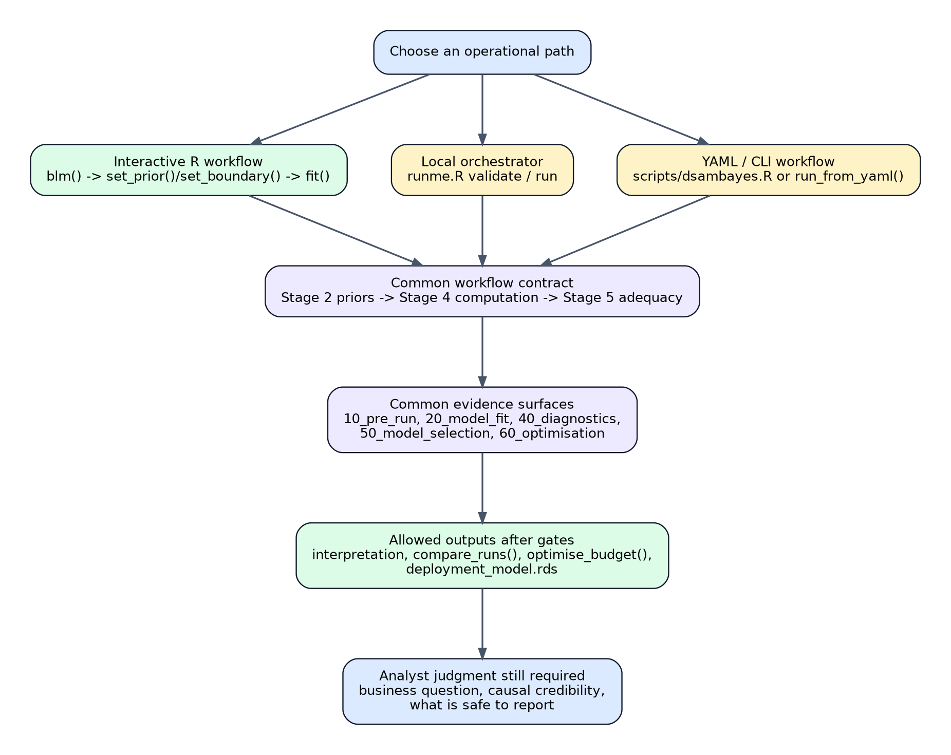
Workflow vectors
Different operational entry points in DSAMbayes still converge on the same
workflow contract. Whether you work interactively in R, use runme.R, or run
the YAML / CLI path, the result should still pass the same prior, computation,
and adequacy gates before interpretation.
fit plots, PPC, residual diagnostics, LOO/Pareto-k
Do not use decomposition or optimisation for decisions
Interpretation and decision
Are we reporting uncertainty and caveats honestly?
decomposition, response curves, optimisation
Restrict or block business use
Two rules to remember
1. Passing sampler diagnostics is necessary, not sufficient
Good Rhat, ESS, and zero divergences mean the posterior draws are numerically credible. They do not prove the model is a good description of the data, and they do not prove causal validity.
2. Good fit is not causal proof
A model can fit well, calibrate well, and still estimate the wrong media effects if the identifying assumptions are weak. DSAMbayes can make the workflow more disciplined; it cannot remove the need for analyst judgment.
How this section relates to the rest of the docs
Workflow pages answer “what should I do and why?”
How-to pages answer “how do I perform this task right now?”
Reference pages answer “what exactly does this field, function, or plot mean?”
Define what DSAMbayes means by a principled Bayesian MMM workflow.
The term is intentionally about process, not brand loyalty to a particular model class or sampler. A principled workflow is one where assumptions are explicit, diagnostics are stage-gated, and downstream interpretation is conditioned on those gates.
The short definition
A DSAMbayes workflow is principled when it does all of the following:
states a clear modelling objective and decision context
specifies an explicit model with explicit priors and boundaries
checks whether the posterior computation is trustworthy
checks whether the fitted model is adequate for the data
carries uncertainty and gate status into decomposition, optimisation, and reporting
If any one of those steps is skipped, the workflow becomes less defensible even if the final coefficients look plausible.
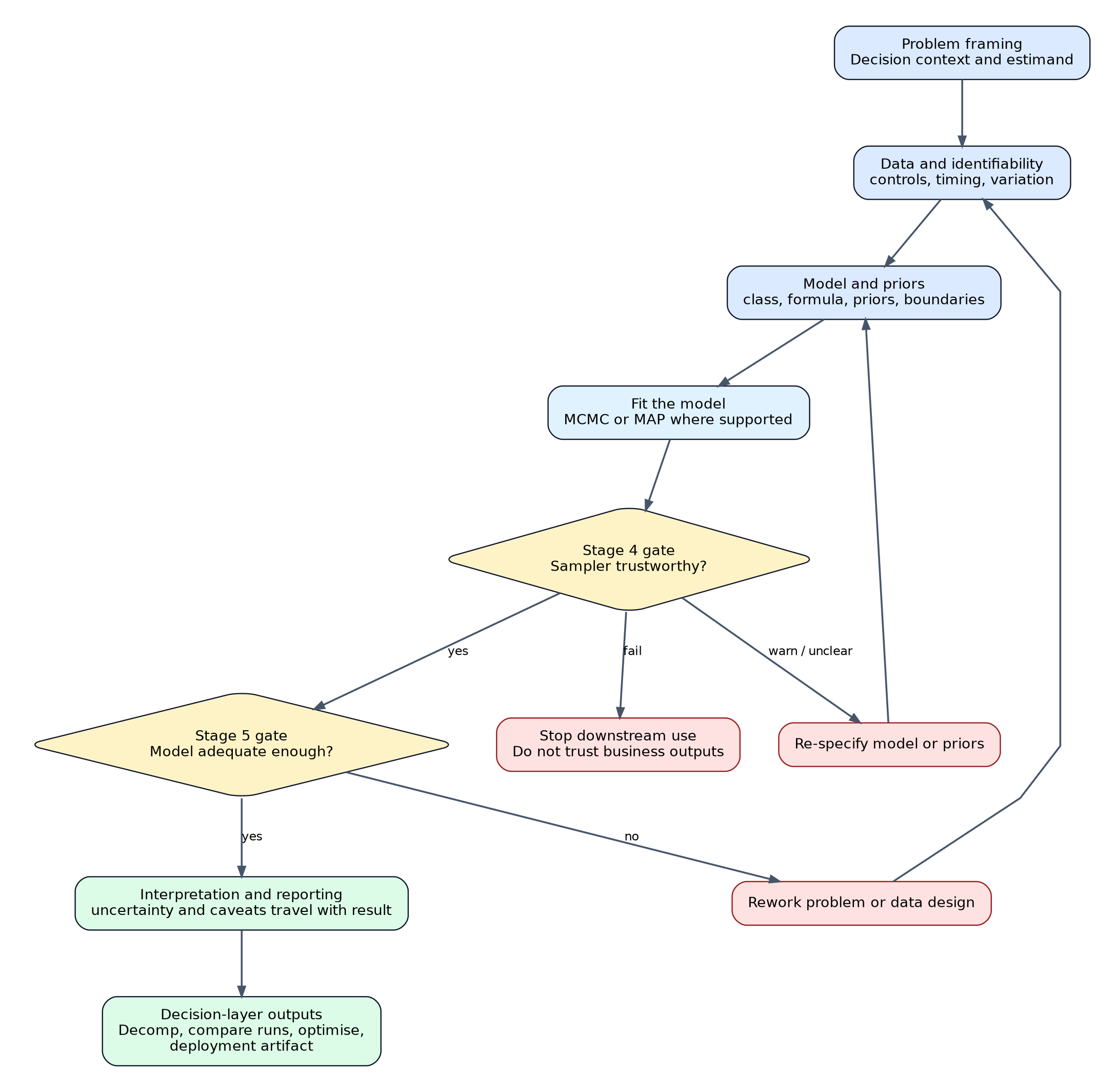
Workflow contract at a glance
The key design choice in DSAMbayes is that downstream outputs are conditional on
upstream gates. A model that fits is not automatically a model that should be
decomposed, compared, optimised, or deployed.
Four commitments
1. Generative transparency
The model should tell a clear story about how the outcome is generated from:
media terms
baseline structure
controls
observation noise
That is why DSAMbayes exposes priors, boundaries, response scale, CRE terms, time components, and model classes explicitly. The point is not to burden users with knobs; it is to make assumptions inspectable.
2. Stage-gated inference
The workflow should move in order:
question and data design
model and priors
fit
computational diagnostics
model adequacy checks
interpretation and decision support
Downstream outputs should only be trusted if the upstream gates have been checked.
3. Diagnostic sufficiency for computation, not causality
Diagnostics answer questions like:
did the sampler converge?
are the posterior draws stable?
does the fitted model describe the observed data credibly?
Diagnostics do not answer:
did the model identify the true causal effect of media?
did we control for every relevant confounder?
is the chosen baseline structure the only defensible one?
This distinction is essential in MMM.
4. Decision-linked reporting
Decomposition shares, response curves, deployment artifacts, and budget recommendations should be treated as functions of the gated fit, not as standalone truths. If the fit has warnings or failures, those limitations must travel with the result.
The three layers of trust
DSAMbayes users should separate three different questions:
Layer
Question
Typical evidence
Computational faithfulness
Are the draws numerically trustworthy?
Rhat, ESS, divergences, treedepth, BFMI
Model adequacy
Does the model describe the observed data credibly?
Passing the first layer does not imply the second. Passing the second does not imply the third.
How DSAMbayes supports this workflow
DSAMbayes already provides several pieces of the workflow contract:
explicit model classes and response-scale semantics
default priors plus selective overrides and hard boundaries
pre-flight design checks
post-fit diagnostics with pass / warn / fail statuses
staged runner artifacts under results/
model comparison and optional time-series selection tooling
decision-layer optimisation with uncertainty-aware summaries
What the package cannot do automatically is replace analyst judgment about:
business estimands
causal assumptions
whether a structural prior is genuinely defensible
whether a warned run is acceptable for the specific business use
Failure policy in plain language
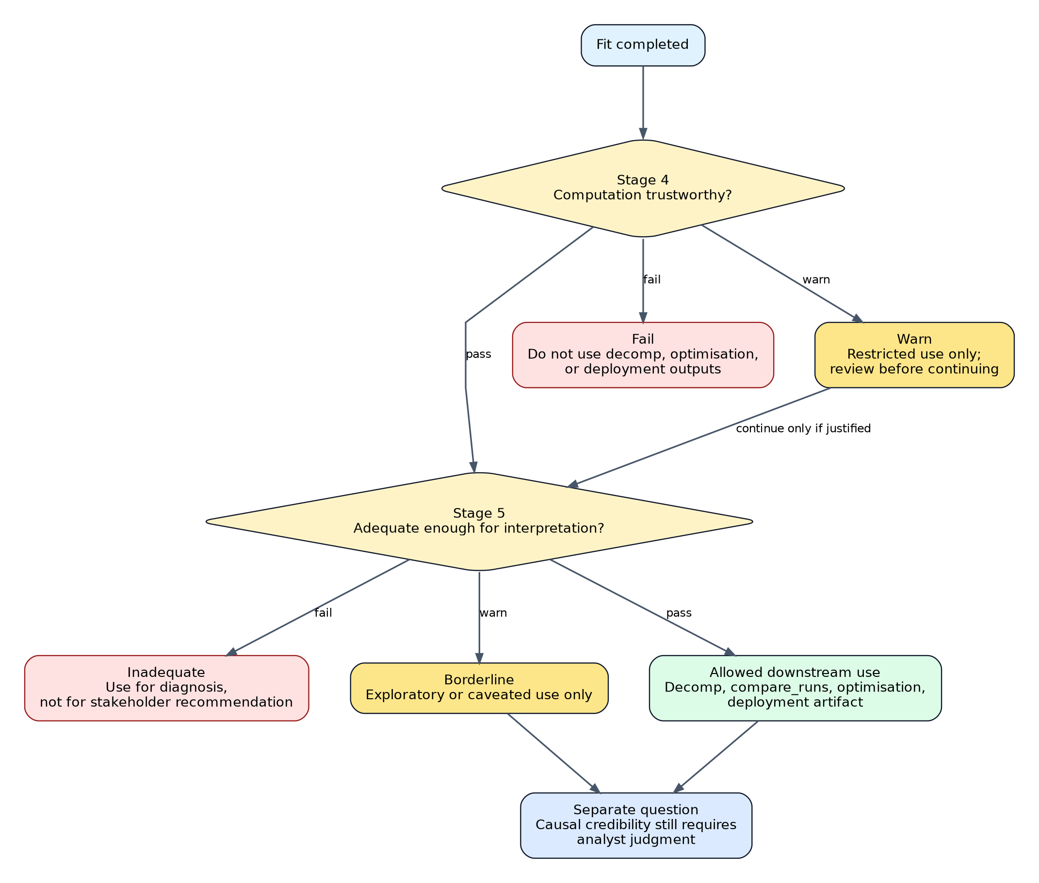
If Stage 4 fails
Do not trust decomposition, response curves, or optimisation outputs. The posterior sample itself is numerically unreliable.
If Stage 5 fails
The sampler may have worked, but the model is not yet adequate for business interpretation. Use the run for diagnosis, not for stakeholder recommendations.
If causal assumptions are weak
Even a clean computational and adequacy profile may still only support associational interpretation. Report it that way.
Translate familiar classical regression instincts into the DSAMbayes workflow so users coming from OLS, GLM, or general frequentist econometrics can adopt Bayesian MMM without losing methodological discipline.
What does not change
Moving to DSAMbayes does not remove the need for:
careful data definition
sensible controls
thinking about omitted variables
residual scrutiny
skepticism about causal claims
Bayesian MMM is not a shortcut around model design. It is a different way of expressing assumptions and uncertainty.
What changes
1. From one best coefficient to a posterior distribution
In OLS, the default object of interest is a point estimate plus a standard error.
In DSAMbayes, the default object is a posterior distribution. That means:
coefficients are uncertain objects, not fixed truths
decomposition and optimisation should inherit that uncertainty
wide intervals are information, not a nuisance to hide
2. From “no prior” to “explicit prior assumptions”
Frequentist workflows often treat themselves as prior-free. In practice, they still encode structure through model choice, variable transformations, and constraints.
DSAMbayes makes that structure explicit:
default priors express mild regularisation
boundaries express structural sign assumptions
overrides should be sparse and justified
3. From significance-thinking to decision-thinking
The key question becomes less “is beta significantly different from zero?” and more:
is the posterior sufficiently stable?
is the model adequate?
is the interval narrow enough for the business decision?
what risks remain if we act on this estimate?
Quick translation table
Frequentist instinct
DSAMbayes replacement
“Run the regression and inspect coefficients”
Specify the model, priors, and boundaries, then inspect the full posterior
“Use p-values to screen variables”
Use posterior intervals, sign stability, and workflow diagnostics
“Choose the model with the best fit statistic”
Choose among models that first pass diagnostics and then compare predictive evidence
“If the model converged, the answer is credible”
Convergence is only the computation gate; adequacy and interpretation are separate gates
“No prior means unbiased starting point”
Defaults are still assumptions; make them explicit and inspect whether they are defensible
“A high R-squared validates the model”
Fit can be good while causal interpretation remains weak
The priors question in frequentist language
The question “where do priors come from?” is often really one of these:
What assumptions am I already making implicitly?
Which assumptions deserve to be encoded explicitly?
Where do I have stable directional knowledge versus weak intuition?
For DSAMbayes, the practical default is:
start with package defaults
add boundaries only for structural signs you would defend in writing
add sparse prior overrides only for high-conviction terms
do not use priors to force a preferred answer out of weak data
Default priors are a sensible starting point, not proof that prior design is solved forever.
Mistake 2: using priors as a repair tool for poor design
If media terms are badly collinear with baseline structure or controls are missing, stronger priors may stabilise numerics without fixing the underlying modelling problem.
Mistake 3: treating warning-level diagnostics as a cosmetic issue
A warned run may still be usable, but only if the warning is understood and disclosed. The right response is not “the model ran, so ship it.”
Mistake 4: confusing predictive success with causal proof
A model can rank well by ELPD and still be causally fragile.
Practical recommendation
If you are used to classical MMM, use DSAMbayes in this order:
Specify a model that is explicit enough to be audited and simple enough to be defended.
For most DSAMbayes users, this stage is where the biggest conceptual shift happens. In classical MMM, the common instinct is to choose variables, run the regression, and worry about coefficient stability afterwards. In DSAMbayes, priors and boundaries are part of the specification from the start.
The operating rule
Use a default-first workflow unless there is a strong reason not to.
That means:
start with the package defaults
add sparse sign constraints only where the business logic is structural
add sparse prior overrides only where the prior story is stable and defensible
fit the model
inspect whether the posterior is still dominated by weak design rather than by a sensible prior choice
This is the same operating stance documented in Minimal-Prior Policy, but framed here as part of the modelling workflow rather than as a standalone policy page.
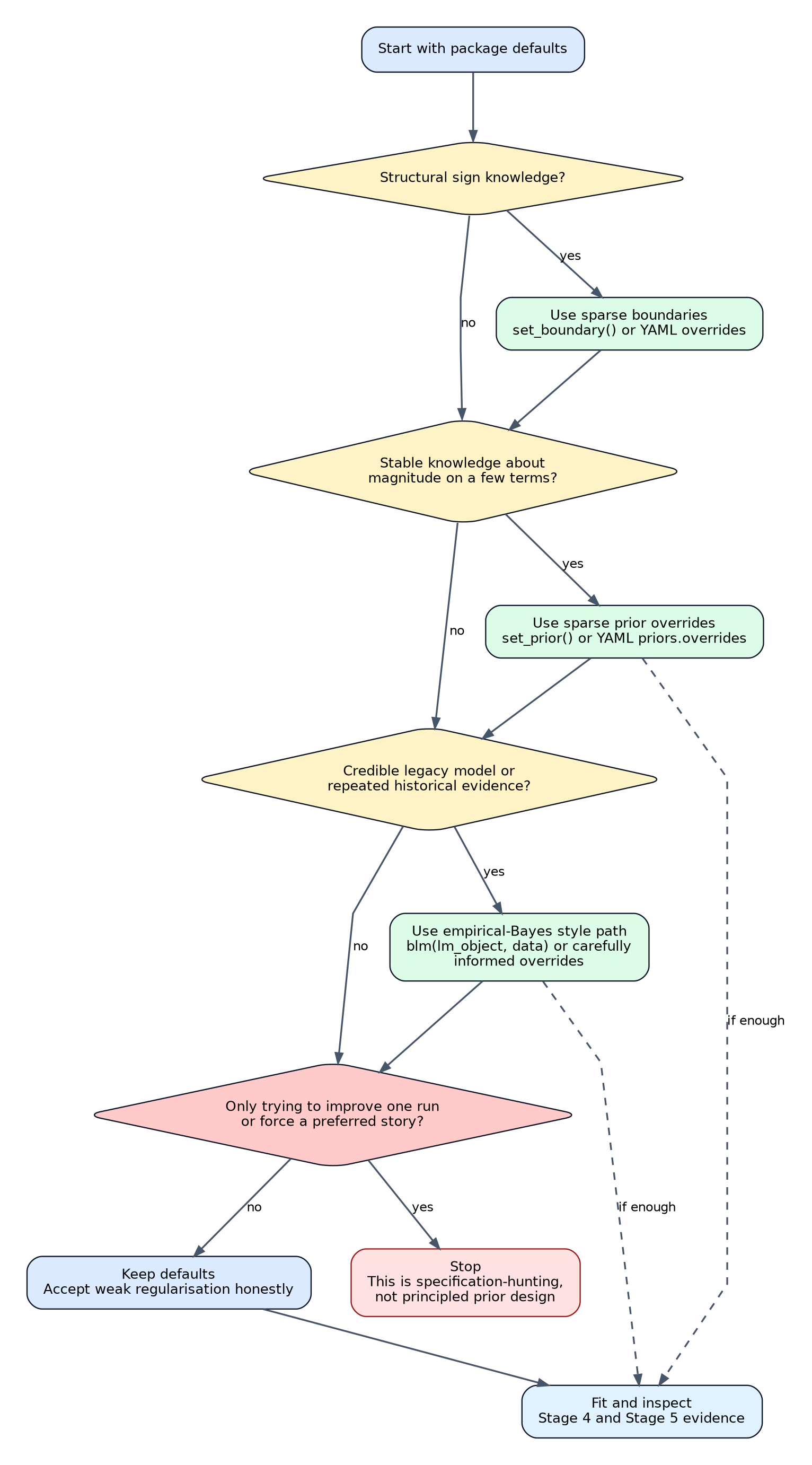
Prior specification pathways
This is the short answer to “where should priors come from?” Defaults are the
starting point. Boundaries and overrides are additive, sparse, and justified by
business or structural reasoning. The blm(lm_object, data) path is the
empirical-Bayes-like option when a credible legacy model already exists.
Where priors should come from
In DSAMbayes, priors should usually come from one of four sources.
1. Structural sign knowledge
Examples:
additional media exposure should not reduce KPI
competitor discount should not increase our sales
This is usually best expressed as a boundary, not as an aggressive mean-shifting prior.
2. Stable business knowledge about magnitude
Examples:
price elasticity is probably negative and modest
distribution is probably positive and not enormous
This is where a sparse override like normal(-0.2, 0.1) may be justified.
3. Historical learning from previous analyses
If the same brand, market, or response has been analysed repeatedly under a similar data-generating regime, you may have enough evidence to justify informative priors on a small number of terms.
4. Explicit regularisation when the data are weak
Sometimes priors are primarily there to stabilise a short, collinear MMM. That is acceptable, but it should be acknowledged honestly as regularisation rather than presented as deep subject-matter certainty.
Where priors should not come from
Do not set priors mainly because:
one previous run looked better with them
they remove a warning without improving model design
they force a preferred channel ranking
they make weak data look more certain than it really is
That is specification-hunting, not principled prior design.
Practical DSAMbayes policy
Step 1: start with defaults
For most first-pass BLM and hierarchical work, the package defaults are the right starting point.
default coefficient priors are weakly informative
default boundaries are unconstrained
you should not feel obliged to invent bespoke priors on every term
Step 2: add selective boundaries
Use set_boundary() or YAML boundaries.overrides when the sign is structural and defensible.
Good examples:
media terms constrained positive
competitor discount constrained non-positive
Poor examples:
constraining every control just to reduce posterior variance
forcing signs on variables whose mechanism is genuinely ambiguous
Step 3: add sparse prior overrides only where conviction is real
Typical candidates:
price
distribution
a small number of strategically important baseline controls
Typical non-candidates:
every media term
every generated seasonal component
every term simply because the data are noisy
Step 4: keep the reasoning on the original outcome scale
DSAMbayes can scale internally when scale = TRUE, but your reasoning about priors should still happen on the original business scale. Ask:
what outcome change would this prior imply?
would that be plausible for this KPI?
would I be comfortable defending it in a model review?
Prior predictive discipline in DSAMbayes
The Bayesian workflow ideal is to inspect prior implications before posterior fitting. In practical DSAMbayes use today, that discipline is still partly analyst-driven.
v1.3.3 does not yet provide a fully productised, first-class prior-predictive runner stage with its own public gate contract. So the current disciplined approach is:
keep the prior design simple
reason on the original outcome scale
avoid over-confident overrides unless they are well supported
fit the model and then inspect whether the posterior behaviour is compatible with the prior story and the data
That makes the lack of a first-class prior-predictive stage a reason to be more conservative, not less.
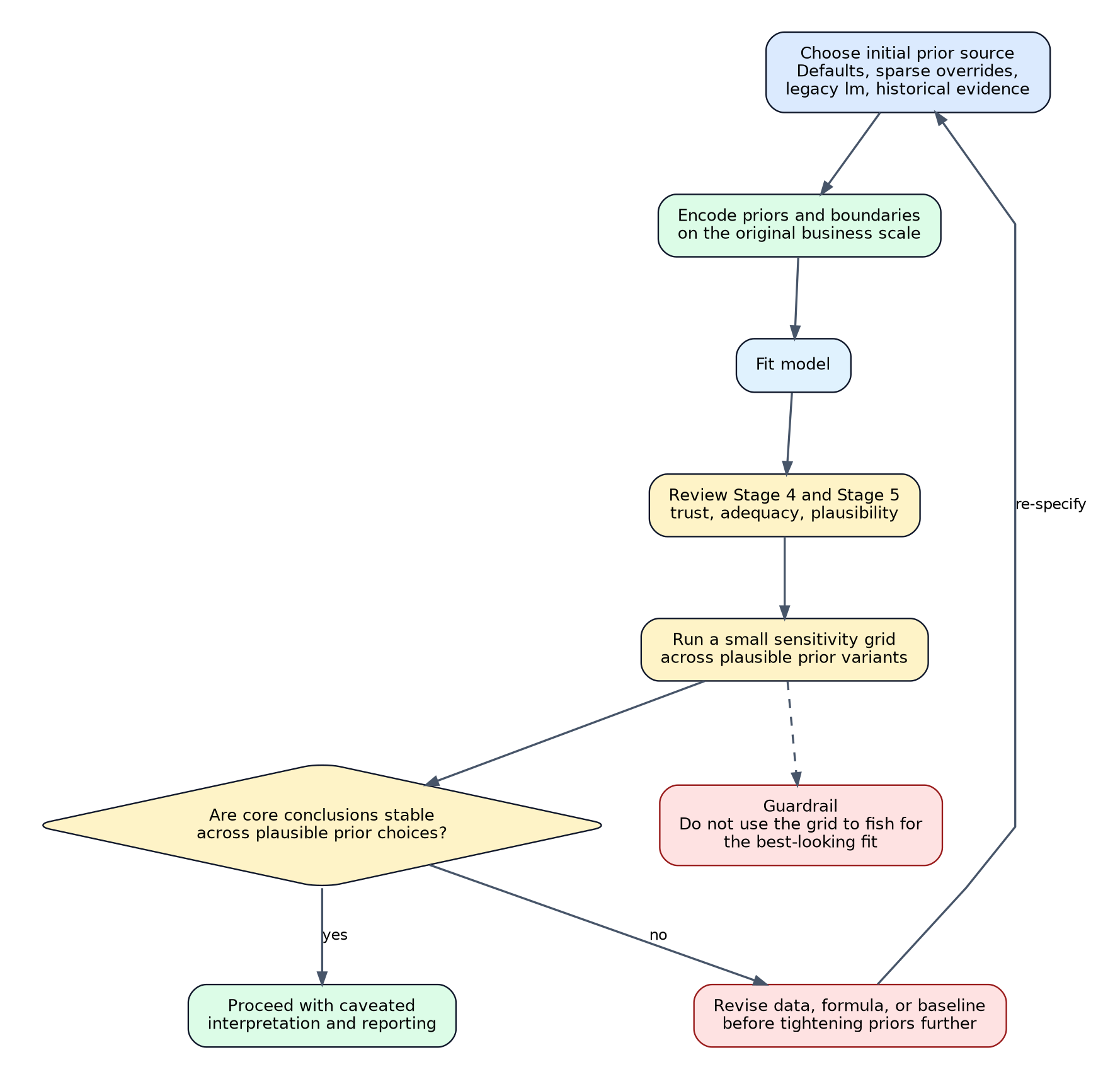
Prior calibration and sensitivity loop
For DSAMbayes users, a prior grid is a robustness tool, not a scoring contest.
Use it to check whether the substantive conclusion survives plausible prior
choices. Do not use it to hunt for the prior that makes one run look best.
How to know whether the priors are doing sensible work
After fitting, ask:
Are the intervals still wide?
If yes, the data may simply be weak. Do not respond automatically by tightening priors.
Are signs unstable without a clear design reason?
Check the baseline structure, controls, collinearity, and response-scale choice before strengthening priors.
Are coefficients pinned to hard bounds?
That can indicate that the boundary is too strong, or that the model is trying to express a structure the current formula does not support well.
A simple prior-setting decision table
Situation
Recommended action
First pass on a standard MMM
Use defaults, then add only obvious sign boundaries
Strong business reason for one control sign or magnitude
Add one sparse override or boundary
Weak identification and high collinearity
Diagnose design first; do not immediately tighten priors
Short dataset with many channels
Accept that intervals may stay wide; simplify model before forcing strong priors
Reviewer asks “why this prior?”
Be able to answer in one sentence on business or structural grounds
Decide whether the posterior draws are numerically trustworthy.
This stage is about computation quality, not business interpretation and not causal validity. If it fails, every downstream quantity that depends on posterior draws becomes unreliable.
The key question
Before asking whether the model is good, ask whether the sampler actually explored the posterior well enough for the summaries to mean what they appear to mean.
In DSAMbayes, this is the stage where you care most about:
divergences
Rhat
effective sample size
treedepth and BFMI when available
Recommended order of attention
1. Divergences
Any non-zero divergences should be treated seriously. They are often the strongest sign that the sampler struggled with posterior geometry.
Typical actions:
increase adapt_delta
simplify the model
revisit boundaries or extreme prior choices
inspect whether a hierarchical structure is too ambitious for the data
2. Rhat
Rhat answers: did the chains mix into the same posterior region?
Practical rule:
at or below 1.01 is the target
above 1.01 fails the publish and strict diagnostics policies
3. Effective sample size
ESS answers: how much independent information do the posterior summaries really contain after accounting for autocorrelation?
Low ESS means:
interval estimates may be unstable
tail probabilities may be noisy
apparent posterior precision may be misleading
4. Treedepth and BFMI
These are geometry warnings. They often indicate a difficult posterior shape even when Rhat looks acceptable.
What DSAMbayes gives you
You can inspect this stage through:
chain_diagnostics(model) for interactive fitted models
40_diagnostics/diagnostics_report.csv
40_diagnostics/diagnostics_summary.txt
diagnostics plots and residual artifacts produced by the runner
Decide whether the fitted model is a credible description of the observed data.
This is the stage that sits between computational trust and business interpretation. A model can pass sampler diagnostics and still fail here.
The key question
If I simulate from the fitted model, does it reproduce the important structure of the observed data well enough for decomposition, comparison, and optimisation to be taken seriously?
What to inspect first
1. Fitted-versus-observed behaviour over time
Ask:
does the model track the broad level and movement of the KPI?
are there long runs of systematic over- or under-prediction?
are key seasonal or event patterns still unexplained?
2. Posterior predictive checks
Posterior predictive plots tell you whether the fitted model can generate data that look like what you observed.
In DSAMbayes, this is the right way to think about the ppc.png artifact: not as decoration, but as an adequacy check.
3. Residual behaviour
Residual autocorrelation or visible structure usually means the model has not absorbed an important baseline, timing, or event component.
4. LOO and Pareto-k
Model comparison and calibration-style plots help answer:
which candidate model predicts better?
are some observations highly influential?
is the leave-one-out approximation trustworthy?
These are useful, but they should not override a bad adequacy profile.
What this stage means for decisions
The main practical consequence of Stage 5 is that predictive ranking and
downstream business outputs are conditional on adequacy. Passing computation
checks is not enough if the fitted model still behaves poorly against the data.
If adequacy is poor
Do not interpret decomposition shares as if they were stable statements about media contribution.
Do not treat optimisation outputs as reliable budget guidance.
Use the run to diagnose misspecification, then revise the model.
If adequacy is acceptable but not clean
A warning-level result may still be useful for exploratory work, but the caveat should travel with the output.
Adequacy is not the same as causality
A model can:
fit well
calibrate well
compare well by predictive metrics
and still produce biased media-effect interpretation if confounding or structural misspecification remains.
So Stage 5 is a gate on model adequacy, not proof of causal validity.
Practical DSAMbayes reading order
Check Stage 4 first: are the draws trustworthy?
Inspect fit plots and PPC
Inspect residual diagnostics
Inspect LOO / Pareto-k and compare candidate runs
Only then interpret decomposition or decision-layer outputs
Common failure patterns
Pattern 1: good convergence, bad residual structure
Interpretation: the sampler worked, but the baseline or control structure is incomplete.
Pattern 2: good fit plot, unstable influential observations
Interpretation: apparent adequacy may depend too heavily on a small number of points. Treat model comparison and downstream interpretation cautiously.
Pattern 3: good predictive fit, weak causal story
Interpretation: the model may be operationally useful for forecasting or scenario analysis, but not for strong causal claims about media.